Confinement in Toy Models
The abelian Higgs model
The usual way to find the spectrum of a model, once given the Lagrangian, is as follows. We write down the Lagrangian in terms of effective degrees of freedom, namely particles, and look for terms that looks like $+\frac{1}{2} m^2 \phi^2$, where $\phi$ is the degree of freedom and $m$ would be the mass. Then people may carry on to quantize the theory and look for the whole spectrum. However, the non-perturbative effects, especially instantons, which are soliton solutions living in the Euclidean spacetime, might change that picture entirely. For example, originally massless particles might develop mass due to instanton induced effects.
First we look at essentially abelian gauge theory in $1+1$ and $2+1$ dimensions, “essentially” because we also consider the situation where non-abelian symmetries are spontaneously broken to $U(1)$.
Consider in $1+1$ spacetime the Lagrangian,
\[\mathcal{L} = \left\lvert D_{\mu}\phi \right\rvert^2 - \frac{\lambda}{4}(\phi^\ast \phi)^2-\frac{\mu^2}{2}\phi^\ast \phi-\frac{1}{4e^2}F_{\mu \nu} F^{\mu \nu}.\]As for the definition of the covariant derivative, the reader can refer to the note on conventions, which is in agreement with David Tong’s notes. The choice of position of the coupling $e^2$ (in the denominator instead of numerator) also follows from his convention. If you like you can movie $e^2$ to the numerator, which would be the convention preferred in Peskin and Schroeder.
We have a $U(1)$ gauge transformation given by a $U(1)$-valued function $g(x,t)$, for example under the gauge transformation $\phi$ transforms as
\[\phi(x,t) \to g(x,t) \phi(x,t).\]If we require $g(x,t)\mid_{x=\infty} = 0$ at the boundary, then in the eyes of $g(x,t)$, the boundary of space is compactified to a single point. For example, supposed the space is a two dimensional plane, then in the eyes of $g$, the boundary of the plane, namely $\mathbb{S}^1$ is effectively the same as a point, since $g(x,t)$ is force to take the same value everywhere on the $\mathbb{S}^1$, and the topology of the space will be $\mathbb{R}^2$ with its boundary compactified to a single point, namely
\[\mathbb{R}^{2}\cup \text{boundary}\cong\mathbb{S}^2.\]Depend on the sign of $\mu^2$ in the Lagrangian, there are two possibilities. If $\mu^2$ is positive, we have a massive scalar $\phi$ and a massless gauge field $A^\mu$. The interaction is the usual Coulomb interaction. In $1+1$ dimension, the Gauss’s law suggest that the force between two charges does not decrease as the distance increases, consequently it costs infinite energy to separate two charges infinite far away, which is called confinement. Note that different people might use different definitions of confinement and it can by annoying.
In $1+1$ dimensions there is also no photon. An easy way to see this is to go back to the classical electrodynamics, where photons are electro-magnetic waves vibrating in the transverse direction as opposed to its propagating direction. However in 1-dimensional space there is no such thing as “transverse direction”, thus there can be no electro-magnetic wave solutions. This suggests that there is also no photon in $1+1$ dimension.
The spectrum in $1+1$ dimension consists of bound states of particle-antiparticle pairs, which are stable due to the confinement, and the fact that they cannot decay into pair of photons, since there exists no photon.
Where $\mu^2<0$ the potential takes the shape of a double well in $1+1$ dimension, or a Mexico hat in $2+1$ dimension. The spontaneous symmetry breaking has many consequences,
- the scalar particle has mass $\frac{\mu}{\sqrt{ 2 }}$,
- the gauge boson has mass $\frac{\mu e}{\sqrt{ \lambda }}$.
Since the medium of the interaction is massive, we expect a Yukawa-kind interaction, $V(r) \sim e^{ -r/M }$.
Again, this conclusion is altered by instanton-induced effects. Instantons change the force between the particles and imply confinement.
To sum up, in both $\mu^2>0$ and $\mu^2<0$ cases in $1+1$ dimension, the force is independent of the separation, the only difference is that for the case $\mu^2<0$ the force is exponentially smaller.
The Euclidean theory and Finite Action
To have instantons we turn to 2-dimensional Euclidean theory, the Lagrangian is \(\mathcal{L} = \left\lvert D_{\mu}\phi \right\rvert^2 + \frac{\lambda}{4}(\phi^\ast \phi - v^2 )^2 + \frac{1}{4e^2}F_{\mu \nu} F^{\mu \nu}.\) It is comprised of three positive definite terms. The requirement of finite action puts strong constraints on the asymptotic behavior of the fields. For instance, the gauge field must go to a pure gauge as $r\to \infty$,
\[A_{\mu} \to g(\theta)\partial_{\mu}g^{-1}(\theta), \quad g\in U(1).\]The function $g(\theta)$ gives a map from the boundary of $\mathbb{R}^2$, namely $\mathbb{S}^1$ into the group $U(1)$, that is
\[g: \partial \mathbb{R}^2 \cong \mathbb{S}^1 \to U(1)\cong\mathbb{S}^1.\]Maps from $\mathbb{S}^1$ to $\mathbb{S}^1$ are classified by the first homotopy group $\pi_{1}(\mathbb{S}^1)$, by winding number $n\in \mathbb{N}$. Given the explicit form of $g(\theta)$, the winding number can be read off from the exponential part, for instance $g(\theta) = e^{ i n \theta }$ has winding number $n$. The winding number can be also calculated using the formula
\[n = \frac{i}{2\pi}\int_{0}^{2\pi} g(\theta)dg^{-1}(\theta) \, d\theta.\]The winding number, like any other topological numbers, are invariant under continuous variance.
The map from $g(\theta)$ to the winding number also maps multiplication to addition, like exponents, where $e^{ a }\times e^{ b }=e^{ a+b }$. To see this, just verify that
\[g(\theta) = g_{n_{1}}(\theta)g_{n_{2}}(\theta) \implies \text{ winding number of }g(\theta) = n_{1}+n_{2}.\]Finally, using $iA_{\mu} = g \partial_{\mu}g^{-1}+\mathcal{O}(1 / r^2)$, we have
\[n = -\frac{1}{2\pi}\int dx^2 \, \partial_{\mu}\epsilon_{\mu \nu}A_{\nu} := - \frac{1}{4\pi}\int dx^2 \, \epsilon_{\mu \nu}F_{\mu \nu}=-\frac{\Phi}{2\pi},\]where $\Phi$ is the flux. The flux in quantized in units of $2\pi$.
Nielson-Olsen Vortices
The solution for each winding number $n$ are known to exist and called the Nilson-Olesen vortices. They are described by two radial functions (the profile functions)
\[A_{\mu} = \epsilon_{\mu \nu} r_{\nu} \frac{\Phi(r)}{2\pi r^2}\]for the gauge field and
\[\phi(t) = e^{ i\theta }f(r)\]for the scalar field. Substitute them in the equation of motion we will have the equation of motion in terms of $\Phi$ and $f$. A solution exists, the shape of the profile functions can be found easily online so we won’t present it here.
The interesting part is that the solution actually has non-zero magnetic field! Recall that the magnetic field can be written in terms of $A_{\mu}$ and now $A_{\mu}$ is given in terms of $\Phi(t)$, thus we can write down the magnetic field in terms of $\Phi(t)$, after some derivation we have
\[B(r) = \frac{1}{2\pi r} \frac{d}{dr} \frac{\Phi(r)}{2\pi} \to C e^{ -erf(r) }.\]The boundary condition is that
\[\begin{align} f(r) & \to a, \\ \Phi(r) & \to \Phi. \end{align}\]$\Phi(r)$ has the interpretation of being equal to the magnetic flux inside the radius $r$ while $\Phi$ is the total magnetic flux in the soliton, which is quantized in units of $2\pi$.
The magnetic field is concentrated around the origin and decreases exponentially outwards.
Remember that one of the 2 dimensions was originally time, thus going back to the Minkowski spacetime, the instanton solution spans in both space and time. The instanton solution mediates between two topologically different vacuums, both with zero energy. Where does the degenerate vacua come from? To answer that question, first we need to take a look at the Hamiltonian (energy) density.
Switch back to the Minkowski metric. In the $A_{0} = 0$ gauge (sometimes called the temporal gauge), the energy is given by
\[\mathcal{E} = \int dx \, \frac{1}{2e^2} (\partial_{0}A_{1})^2 + \left\lvert \partial_{0}\phi \right\rvert^2 +\left\lvert D_{1}\phi \right\rvert^2 + \lambda(\phi^\ast \phi)^2.\]An obvious vacuum is $A = 0, \phi = v$, which we call the trivial vacuum. However, don’t forget that the model has $U(1)$ gauge symmetry, hence any gauge transformation of the trivial vacuum is itself another vacuum. You might ask, but haven’t we already adopted the temporal gauge, thus fixing the gauge altogether? Yes and no. The time-component of the gauge field is fixed, but the space component is not. We still have the freedom to fix the gauge in the spatial direction!
We impose the additional condition,
\[\lim_{ x \to \infty } g(x) = 1.\]This will force the function $g(x)$ to see the 1-D space as a circle. What I mean here is that, since $g(x)$ takes the same value on both ends, we can compactify the two ends of spatial direction $\mathbb{R}$ and make it into the circle, as far as $g(x)$ is concerned, they are the same. Since $g(x)$ takes value in $U(1)\cong \mathbb{S}^1$, the map
\[g:\mathbb{S}^1 \to \mathbb{S}^1\]is again classified topologically by the homotopy group, by winding numbers. In other words, the classical vacua
\[\begin{align} \phi &= g_{n}(x) v, \\ A_{1} &= ig_{n}^{-1}(x)\frac{d}{dx} g_{n}(x) \end{align}\]are indexed by winding number $n\in\mathbb{N}$ and different vacua are homotopy inequivalent.
However, unlike in the double well QFT model, the transition amplitude from one vacuum to another is not infinite anymore, for the energy barrier between them are now finite. This is because we can find a finite action solution in the Euclidean spacetime. The Nielson-Olesen vortices interpolate between these vacua. This is not supposed to be obvious the the naked eyes though, to see that we first need to convert the Nielson-Olesen vortices into the temporal gauge.
We can approximate the spacetime, whether Euclidean or Minkowski, as a square, where the $x$-axis is space and $y$-axis is the time. We call it the spacetime square.
We first perform a gauge transformation $g(\theta)=e^{ -i\Lambda(\theta) }$. We can construct a function $\Lambda(\theta)$ such that it is topological trivial on the boundary of spacetime square, $\partial\mathbb{R}^2$ so that it can be continuated to everywhere on the square, and the resulting gauge field satisfy
- At the past, namely the bottom line of the spacetime square, the gauge field is zero everywhere,
- at the future boundary, namely the top line of the square, the gauge field $A_{1}$ is not zero but $A_{0}$ is zero, as required by the temporal gauge.
As the result, we can put the Nielson-Olesen vortex in a gauge such that all the nontrivial winding only appears in the spatial line $x$ at the top line of the spacetime square.
The Nielson-Olesen vortex now interprets between two different vacua,
- at the past boundary is the trivial vacuum, $g(x) =1$,
- at the future boundary, the vacuum is given by some gauge transformation $g(x) \neq 1$.
Tunneling transition
We can calculate the matrix element
\[\left\langle n \right\rvert e^{ -HT/\hbar } \left\lvert{0}\right\rangle = \mathcal{N}\int_{\nu[\phi_{\text{in}}]=0}^{\nu[\phi_{\text{out}}]=n} \mathcal{D}A_{1} \mathcal{D}\phi^\ast \mathcal{D}\phi \, e^{\frac{-S_{E}[\phi]}{\hbar}}\]using semi-classical methods. The functional integral is over all the field configurations with winding number $n$. This of course includes the configuration with one instanton with winding number $n$, but that is by no means the only, or even the most important, configuration. There could as well be $n_{+}$ instantons with winding number $1$ and $n_{-}$ anti-instantons with winding number $-1$. Assume these instanton and anti-instantons are separated far enough (the so-called instanton gas model) so the total configuration can be approximated by simple superposition of single instanton solutions. The action should include
- configurations with action $(n_{+}+n_{-})e^{ -S[\text{ins}] }$, where $S[\text{ins}]$ is the action of a single $n=\pm 1$ instanton, and
- There is a entropy factor summing over all the possible locations of the instantons, $\frac{(TL)^{n_{+}+n_{-}}}{(n_{+})! (n_{-})!}$.
Long story short, by calculating the transition amplitude, also with the help of identity
\[\delta_{a,b} = \frac{1}{2\pi}\int_{0}^{2\pi} d\theta \, e^{ i\theta(a-b) }\]we find that the real vacua with the presence of instantons are label by $\theta$ angle, with energy
\[{\mathcal{E(\theta)}} = -2KL\,e^{ -S_{0}/\hbar }\cos \theta\]Remarks.
- The total energy assigned with each $\theta$ is proportional to the total volume, as expected.
- Theta-energy is proportional to $\cos \theta$
- Due to the $e^{ -S_{0} }$ factor, it is exponentially suppressed.
The matrix element
\[\langle n \mid \theta \rangle =\frac{e^{ i n \theta }}{\sqrt{ 2\pi }}.\]The Wilson loop
The rearrangement of the vacuum has important consequences for the force between charges. A charged particle, when moving in the electromagnetic field, along the way acquires a phase
\[e^{ -iq/e \int dx_{\mu} \, A_{\mu} }\]where $q$ is the charge of the particle and $\frac{q}{e}$ is dimensionless. To see this, consider an charged particle governed by the gauged Lagrangian
\[L = \frac{1}{2} \dot{x}^2 + q \dot{x}_{i} A_{i} -qA_{0} - V(x_{i}),\]From the Lagrangian we get the equation of motion where the particle is coupled to the gauge field. The gauge field can also be written in terms of electric and magnetic fields. Thus, in comparison to the not-gauged case, the now gauged path integral is augmented by the extra gauge-coupling term
\[\boxed{ e^{ -i S_{0}/\hbar } = (\text{old terms}) \times e^{ -i \frac{q}{e} \int dt \,(A_{0}-\dot{x}_{i}A_{i}) } = (\text{old terms}) \times e^{ -i \frac{q}{e} \int dx^\mu A_{\mu}}. }\]For an antiparticle we just need to change the sign of the charge.
Next we introduce one of the most important concepts in quantum field theory, the Wilson loop, which is indispensable in the study of confinement, or interactions in general, in any quantum field theoretic model.
Imagine that we create a pair of charged particles from the thin air. These test particles are put in by hand, their position and motion fixed by hand. They behave as we want them to, yet still coupled to the gauge fields, experiencing all the interactions. They are sometimes referred to as external charges. So, after we create the pair, we force them to separate by a large distance $R$. Then we hold the particles fixed for time $T’$, so they could have a long enough time to fully appreciate the interaction between them. After time $T’$, we send them back to where they were created and annihilate them into nothing, dust to dust. The trajectory of these two particles will form a loop, as shown in the below. It is the Wilson loop.
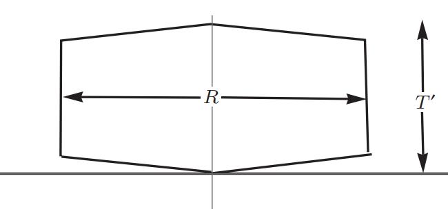
Now the question is: for the Wilson loop shown above, what is the phase factor associated? The phase factor is integrated along the trajectory, which is a closed loop in our case, thus the integral becomes a closed integral,
\(\text{Phase factor } = e^{ -i \frac{q}{e}\oint dx^\mu A_{\mu}} = e^{ -i \frac{q}{e} \oint A }, \quad A := A_{\mu}dx^\mu.\) The associated operator
\[W = e^{ - \frac{q}{e} \oint A }\]is called the Wilson operator. The vacuum expectation value (VEV), also called the matrix element, of Wilson operator can be compared to the time evolution of a pair of (anti-)particles and annihilate them after time $T$, in the language of Hamiltonian is proportional to $e^{ - Ht }$, the minus sign since we are now working in the Euclidean metric. Thus the VEV of Wilson loop has the interpretation of $e^{ -E(R)T }$, where $E(R)$ is the energy of a particle-antiparticle pair separated by distance $R$.
If $E(R)\sim cR$ for some constant $c$, the interaction between two charges is said to be confining, since the energy needed to separated them increases linearly with distance, eventually the energy between then will be enough to create another pair of particle-antiparticle. The VEV of Wilson loop operator will behave like
\[\left\langle W \right\rangle \sim e^{ -c A }\]where $A$ is the area of the loop. This is the celebrated area law criterion of area law behavior of the Wilson loop for confining interactions.
If the potential behaviors like $E(r)\sim D$ for some constant D, we get
\[\left\langle W \right\rangle \sim e^{ -DT }\sim e^{ -D(2T)/2 }\sim e^{ -D (2T+2R)/2 }\sim e^{ -D'P }\]where $D’$ is some constant and $P$ the perimeter of the loop. Such behavior is called the perimeter law, and does not imply confining interactions.
VEV of Wilson loop in instantons background
Since the behavior of Wilson loop show whether the system is confined or not, we want to evaluate the expectation value of it in the theta vacuum, so we would know what effects can instanton gas has to the confinement,
\[\bra{\theta} W \ket{\theta} = \frac{1}{Z_{\theta}}\int D[A_{\mu},\phi^\ast ,\phi] \, e^{ -S_{E} }e^{ i\nu \theta }\;W\]where $S_{E}$ is the Euclidean action, and since we are working in the Euclidean metric, the field configuration with winding number $n$ contribute a factor $e^{ i\nu \theta }$ instead of $e^{ \nu \theta }$, notice the difference of a factor of $i$. $Z_{\theta}$ is the partition function in the background of $\theta$-vacuum, which we will just call theta-vacuum. You might be wondering why there is a factor $e^{ i\nu \theta }$ in the integrand, to understand why, we must first determine the form of the partition function.
The partition function in the background of theta vacuum is
\[Z_{\theta} = \sum_{n} Z_{n}e^{ i n \theta },\quad Z_{n} = \int_{\nu=n} D[A_{\mu},\phi^\ast ,\phi]e^{ -S_{E} } ,\,\]To simplify the notation we could write
\[Z_{\theta} = \int D[A_{\mu},\phi^\ast ,\phi]e^{ -S_{E} }e^{ i n \theta }\]which means that we integrate over all the field configurations, each configuration has a winding number $n$, and contributes a factor $e^{ i n \theta }$ accordingly.
This is also the reason why we have the same factor $e^{ i\nu \theta }$ in Eq. (1). Simply put it, the $e^{ i\nu \theta }$ factor is there because we are evaluating stuff in the theta vacuum.
Now, the expectation value of the Wilson loop is the vev of
\[e^{ -iq\int_{D} \, F_{12}d^2x } = e^{ 2\pi q \nu_{in} }\]where we have used the expression for winding number
\[\nu = -\frac{1}{2\pi}\int d^2x \, F_{12}\]and $\nu_{in}$ is the number of instantons in the domain circled by the Wilson loop.
Equation (2) tells us that, we want to evaluate the expectation value of $e$ to the instanton number in Wilson loop. Given the fact that the average density of instantons is constant in space, clearly the instanton number in Wilson loop is proportional to the area of the loop,
\[\nu_{in} \propto \text{ Area of Wilson loop},\]Thus
\[\left\langle W \right\rangle \sim e^{ \text{Area of wilson loop} }\]and we have the area law! It means that, the existence of instanton gas caused the confinement!
We may also calculate the vev of $F_{12}$ in the background of theta vacuum, using the trick of taking derivatives, which we won’t do here. We claim without proof that
\[\bra{\theta} F_{12} \ket{\theta} \propto \sin \theta \;e^{ -S_E }\]If we have actually calculated the energy between two external charges, (by separating the integral domain into two parts, inside and outside the Wilson loop,) we will find
\[E(R) \propto R \left( \cos(\theta)-\cos\left( \theta+\frac{2\pi q}{e} \right) \right)\;e^{ -S_{0} }\]We notice that the charge of the particle appears in cosine function, thus it is defined modulo $e$, the electric charge of the electron. Physically, it is because between the pair of external particles with charge $q$, pairs of electron with charge $e$ can be created, then can migrate to the opposite charges, neutralizing the external charges. Hence, the charge of the external particles are equivalent modulo $e$. This is caused by the non-perturbative effects.
Enjoy Reading This Article?
Here are some more articles you might like to read next: