Csch Function as a Distributuion
1. $\frac{\sin x}{x}$ as a distribution
Sinc function, or sine cardinal function, also called the sampling function, is an important function in physics and engineering. There are more than one definitions in common use, here we will adopt the following,
\[\text{sinc}(x) = \begin{cases} 1 & x=0 \\ \frac{\sin x}{x} & x\in \mathbb{R}^\ast \end{cases}\]where $\mathbb{R}^\ast := \mathbb{R} \backslash { 0 }$. Thanks to the insertion of $1$ at $x=1$, the sinc function is continuous and smooth on $\mathbb{R}$.
The sinc function, like almost any other functions, defines a distribution, let’s denote it by $T_{\text{sinc}}$. When acted on a function $f$ we have
\[\left\langle T_{\text{sinc}},f \right\rangle := \int_{-\infty}^\infty dx \, \text{sinc} (x)f(x)\]Everything is well defined.
But what about $\frac{\sin x}{x}$ without putting by hand the value $1$ at $x=0$? The function is not defined at $x=0$ so when integrated against some function $f$ we should find a way to circumvent the origin. There are in general two ways to do that, first is by the principal value,
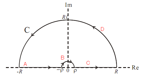
\[\left\langle \frac{\sin x}{x},f(x) \right\rangle := \text{Pv.}\int_{-\infty}^{\infty} dx \, \frac{\sin x}{x}f(x) :=\lim_{ \epsilon \to 0 } \left( \int_{-\infty}^{\epsilon} +\int_{\epsilon}^{\infty} \right)dx \, \frac{\sin x}{x}f(x).\]The other way is to adopt contour integral, the integration goes from $-\infty$ to $\rho$ which is infinitesimal, goes a half-circle above the origin, then goes from $\rho$ to $\infty$. Suppose the integral is zero on the upper infinite half-circle, then we can form a closed loop and the residual theorem can be applied. The contour is shown in the figure below.
Next we shall calculate the Fourier transform of $\sin x / x$ as an example of the two prescriptions. The Fourier transform is
\[\mathcal{F}\left\{ \frac{\sin z}{z} \right\} (\omega) = \int_{-\infty}^{\infty} dz \, \frac{\sin z}{z}e^{ -i\omega z },\]where we change the variable from $x$ to $z$ as a hint that the integral could be carried out on the complex plane.
Let’s try to calculate the first term in the last line using principal value method, then the contour integral.
1.1 Principal value method
We want to evaluate
\(\mathcal{F}\left\{ \frac{\sin z}{z} \right\} (\omega) =\text{Pv.} \int_{-\infty}^{\infty} dz \, \frac{\sin z}{z}e^{ -i\omega z },\) It can be regarded as a distribution defined by $\frac{1}{x}$ acting on a regular function $\sin(z) e^{-i\omega z}$. Note that $\sin(z) e^{-i\omega z}$ is NOT Borel integrable since $\lvert \sin(z) e^{-i\omega z} \rvert$ is not Borel integrable (for details refer to the notes on measure theory) but it doesn’t matter to us. Not being Borel integrable only means that we need to be extra careful when applying, e.g., Fubini’s theorem to the integral.
The problem is that $\frac{1}{x}$ is not locally integrable, recall that a function is called locally integrable if, around every point in the domain, there is a neighborhood on which the function is integrable, which is clearly not the case for $\frac{1}{x}$ since it is not integrable in the neighborhood of $x=0$.
We can simplify the above integral as follows,
\[\mathcal{F}\left\{ \frac{\sin z}{z} \right\} (\omega) = \text{Pv.}\int_{-\infty}^{\infty} dz \, \frac{\sin z}{z} [\cos(\omega z)-i\sin(\omega z)] =\text{Pv.} \int_{-\infty}^{\infty} dz \, \frac{\sin z}{z} \cos(\omega z)\]since $\sin z / z$ is even, cosine is even and sine is odd. Then the Cauchy principal value is
\[\text{Pv.} \int_{-\infty}^{\infty} dz \, \frac{\sin z}{z} \cos(\omega z) = \lim_{ \epsilon \to 0 } \left( \int_{-\infty}^{-\epsilon} +\int_{\epsilon}^{\infty} \right) dz \, \frac{\sin z}{z} \cos(\omega z) = 2 \lim_{ \epsilon \to 0 } \int_{\epsilon}^{\infty} \frac{\sin z}{z} \cos(\omega z),\]which can be calculated using Feynman’s trick. This trick involved taking derivatives under the integral notation. It goes as follows.
We define a new integral with an extra parameter $\lambda$,
\[H(\lambda) = 2 \lim_{ \epsilon \to 0 } \int_{\epsilon}^{\infty} \frac{\sin z}{z} \cos(\omega z)e^{ -\lambda z },\]clearly $H(\lambda)$ goes to zero if $\lambda$ goes to infinity. We can not calculate $H(\lambda)$ directly but we can calculate the derivative of it with respect to $\lambda$, that is why we defined $H(\lambda)$ as we did. Writing $\cos x$ as $(e^{ ix }+e^{ -x }) / 2$ , we have
\[H(\lambda) = 2 \lim_{ \epsilon \to 0 } \int_{\epsilon}^{\infty} \frac{\sin z}{z} \frac{1}{2}(e^{ i\omega z }+e^{ -i\omega z }) e^{ -\lambda z }:= H_{I}(\lambda) + H_{I I}(\lambda)\]where
\[\begin{align} H_{I}(\lambda) &= 2 \lim_{ \epsilon \to 0 } \int_{\epsilon}^{\infty} \frac{\sin z}{z} \frac{1}{2}e^{ i\omega z } e^{ -\lambda z }, \\ H_{I I}(\lambda) &= 2 \lim_{ \epsilon \to 0 } \int_{\epsilon}^{\infty} \frac{\sin z}{z} \frac{1}{2}e^{ -i\omega z } e^{ -\lambda z } = H_{I}(\lambda)^\ast. \end{align}\]Finally, let’s take the derivative of $H(\lambda)$ w.r.t. $\lambda$, we obtain
\[\begin{align} \frac{d}{d \lambda}H(\lambda) &= 2 \frac{d}{d \lambda} \lim_{ \epsilon \to 0 } \int_{\epsilon}^{\infty} \frac{\sin z}{z} \cos(\omega z)e^{ -\lambda z } \\ &= 2 \lim_{ \epsilon \to 0 } \int_{\epsilon}^{\infty}\frac{d}{d \lambda} \frac{\sin z}{z} \cos(\omega z)e^{ -\lambda z } \\ &= -2 \lim_{ \epsilon \to 0 } \int_{\epsilon}^{\infty} \sin z \cos(\omega z)e^{ -\lambda z } \\ &= -2 \lim_{ \epsilon \to 0 } \int_{\epsilon}^{\infty} \sin z \frac{1}{2}(e^{ i\omega z } + e^{ -i\omega z })e^{ -\lambda z } \\ &= - \lim_{ \epsilon \to 0 } \int_{\epsilon}^{\infty} \sin z (e^{ i\omega z -\lambda z} + e^{ -i\omega z -\lambda z}). \end{align}\]Writing
\[\frac{d}{d \lambda}H(\lambda) = \frac{d}{d \lambda}H_{I}(\lambda) + \frac{d}{d \lambda}H_{I I}(\lambda),\]we just need to calculate one of them since they are complex conjugate to each other. Let’s calculate $d H_{I} / d \lambda$, since $\sin x = (e^{ ix } - e^{ -ix }) / 2i$ we have
\[\begin{align} \frac{d}{d \lambda}H_{I}(\lambda) &= -\frac{1}{2} \lim_{ \epsilon \to 0 } \int_{\epsilon}^{\infty} dz \, \frac{1}{2i} (e^{ iz }-e^{ -iz })e^{ i\omega z }e^{ -\lambda z } \\ &= \frac{i}{4} \lim_{ \epsilon \to 0 } \int_{\epsilon}^{\infty} dz \, \left\{ e^{ z[i(\omega+1)-\lambda] } - e^{ z[i(\omega-1)-\lambda] } \right\} \\ &= \frac{i}{4} \lim_{ \epsilon \to 0 } \left. \left( \frac{e^{ z[i(\omega+1)-\lambda] }}{i(\omega+1)-\lambda} - \frac{e^{ z[i(\omega-1)-\lambda] }}{i(\omega-1)-\lambda} \right) \right\rvert_{\epsilon}^\infty \\ &= -\frac{1}{2} \frac{1}{(i\omega-\lambda)^{2}+1}, \end{align}\]Note that we have taken the $\epsilon \to 0$ limit. What we want to know is the value of $H_{I}(\lambda=0)$, which can be obtained from the identity
\[H_{I}(0) + \int_{0}^{\infty} d\lambda \, \frac{dH_{I}(\lambda)}{d\lambda} = H_{I}(\infty)=0.\]However, here is where the troublesome begins, it is actually nontrivial to calculate the definite integral! I will just throw at your face the useful result,
\[\int_{-\infty+i\omega}^{\infty+i\omega} \frac{ dz }{1+z^{2}}= \begin{cases} 0 & \lvert\text{Im}(z)\rvert>1, \\ \pi & \lvert\text{Im}(z)\rvert<1, \\ \frac{1}{2} & \lvert\text{Im}(z)\rvert=1. \end{cases}\]To obtain this result we need to use the contour integral, then why don’t we use the contour integral at the first place, right? It makes no sense…
Anyway, we have already marched this far and for the sake of completement, let me just write down the result for $H_{I}(0)$. When $\left\lvert \omega \right\rvert<1$, we have
\[H_{I}(0) = \frac{\pi}{2} + \text{arctan}(i\omega) = \frac{\pi}{2} + \text{arctanh}(\omega).\]By substitute $\omega\to -\omega$ we have $H_{I I}$, putting them together we find the arctanh$(\omega)$ term cancels and we have
\[\mathcal{F}\left\{ \frac{\sin x}{x} \right\}(\omega) = \pi \text{ for } \left\lvert \omega \right\rvert <1\]while
\[\mathcal{F}\left\{ \frac{\sin x}{x} \right\}(\omega) = 0 \text{ for } \left\lvert \omega \right\rvert > 1\]and
\[\mathcal{F}\left\{ \frac{\sin x}{x} \right\} (\omega)= \frac{1}{2} \text{ for } \left\lvert \omega \right\rvert = 1.\]The last part is not important at all, since it is defined on $\omega = \pm 1$ which are just two points, they are $\mu$-negligible so don’t contribute anything in the $\int d \omega$ integral.
1.2 Contour integral method
Writing
\[\sin z = \frac{1}{2i} (e^{ iz }-e^{ -iz }),\]we have
\[\begin{align} \mathcal{F}\left\{ \frac{\sin z}{z} \right\} (\omega) &= \int_{-\infty}^{\infty} dz \, \frac{e^{ iz }-e^{ -iz }}{2iz}e^{ -i\omega z } \\ &= \int_{-\infty}^{\infty} dz \, \frac{1}{2iz}e^{ -i(\omega-1) z} -\int_{-\infty}^{\infty} dz \, \frac{1}{2iz}e^{ -i(\omega+1) z}. \end{align}\]There is a pole at $z=0$, which we can by pass with a contour shown in the picture before, for our convenience I copy it here again.

We want the integral on the infinite semi-circle, namely arc D to vanish. If $\omega-1>0$, with the help of Jordan’s Lemma we can show that the integral actually vanishes on D. If $\omega-1<0$ then we will need to choose another contour.
I will not go to details since it can be easily found elsewhere, for example here is a pretty clear note. I just wanna point out that the results are the same as principal value method, and I strongly suggest to start with contour integral in the first place.
2. $\text{csch} (x)$ as a distribution
2.1 Principal value and Hadamard’s method
Like $\text{sinc}(x)$, $\text{csch}(x)=1 / \sinh(x)$ is singular at $x=0$ and defines a singular distribution. Unlike $\text{sinc}(x)$ which approaches a constant at $x=0$, the limit
\[\lim_{ x \to 0 } \text{csch}(x) = \lim_{ x \to 0 } \frac{1}{x} = \infty.\]Due to the the fact that $\text{csch } x$ is an odd function, when integrated against a regular function (recall that a regular function is a single valued function with finite order of derivatives), the final result is finite, thus $\text{csch } x$ defines a singular distribution, which we write as $\text{csch}$ to avoid introducing new notations. To see that, let $\phi(x) \in L^1$ be a test function, and assume $\phi(x)$ has Taylor expansion around $x=0$ with non-zero radius of convergence, we have
\[\begin{align} \left\langle \text{csch },\phi \right\rangle &= \int_{-\infty}^{\infty} dx \, \text{csch}(x) \phi(x) \\ &= \int_{-\infty}^{-\delta} dx \, \text{csch}(x) \phi(x) + \int_{-\delta}^{+\delta} dx \, \text{csch}(x) \phi(x) + \int_{+\delta}^{\infty} dx \, \text{csch}(x) \phi(x) \end{align}\]where $\delta$ is less than the radius of convergence. In the last line, the first and last terms gives the principal value and is supposed to be finite, the divergence comes from the second term, so we expand the test function and $\text{csch}$ around $x=0$,
\[\begin{align} \int_{-\delta}^{+\delta} dx \, \text{csch}(x) \phi(x) &= \int_{-\delta}^{+\delta} dx \, \text{csch}(x) \left( \phi(0) + \sum_{n=1}^\infty \frac{\phi^{(n)}(0)}{n!} x^n \right) \\ &= \int_{-\delta}^{+\delta} dx\, \left( \frac{1}{x}-\frac{x}{6}+ \frac{7x^3}{360}+\dots \right)\left( \phi(0) + \sum_{n=1}^\infty \frac{\phi^{(n)}(0)}{n!} x^n \right) \\ &= \int_{-\delta}^{+\delta} dx\, \left\{ \frac{1}{x}\phi(0) + \mathcal{O}(x^0) \right\} \end{align}\]where we have singled out the singular part at $x=0$. Fortunately the singular part gives zero since $\phi(0)$ is a constant and $\frac{1}{x}$ is an odd function, so
\[\int_{-\delta}^{+\delta} dx\, \frac{1}{x}\phi(0) =0\]and we are left with a finite integral. The same reasoning also applies to $\text{csch}(x)$, thus the distribution can be defined by
\[\boxed{ \left\langle \text{csch },\phi \right\rangle = \int_{-\infty}^{\infty} dx \, \text{csch}(x) [\phi(x)-\phi(0)] }.\]There is a systematic way to separate the infinite part from the finite part in an integral, due to Hadamard, which can be applied to $\text{csch}(x)$. The advantage of Hadamard’s method is it also applies to “more” singular function such as $1 / x^2$.
Hadamard’s finite part
Suppose we want to define a distribution from a singular function $f(x)$. Given a test function $\phi(x)$, the integral $\int dx \, f(x) \phi(x)$ is divergent, so in order to make sense of such integrals, we need to regularize it first.
There are in general more than one way to regularized a divergent integral. Sometimes, it happens that $f(x)$ can be readily written as the derivative of some function,
\[f(x) = \frac{d}{dx} F(x)\]Then the integral can be written as
\[\int dx \, f(x) \phi(x) = \int dx \, F'(x)\phi(x) = -\int dx \, F(x)\phi'(x) + \text{ surface terms}.\]Where we have integrated by part. With any luck, the integral $\int dx \, F(x)\phi’(x)$ will be locally integrable. Here the surface term might be divergent so
\[\begin{align} \left\langle \frac{1}{x}\theta(x),\phi \right\rangle &=\int_{0}^{\infty} dx \, \frac{1}{x} \phi(x) \\ &=\int_{0}^{\infty} dx \, \ln'(x) \phi(x) \\ &= \ln(x)\phi(x)\mid_{0}^\infty - \int_{0}^{\infty} dx \, \ln(x) \phi'(x) \\ &= \ln(0)\phi(0)- \int_{0}^{\infty} dx \, \ln(x) \phi'(x) \end{align}\]where the first term in the last line is divergent, and we have exploited the assumption that $\phi(x)$ decrease fast enough at $x\to \infty$. Throw it away we obtain the so-called Hadamard finite part of the integral $\int dx \,\theta(x)\phi(x) / x$, sometimes written as
\[\mathcal{H.}\int_{0}^{\infty} dx \, \frac{1}{x} \phi(x) := - \int_{0}^{\infty} dx \, \ln(x) \phi'(x).\]Sometimes the singular function defined by its Hadamard finite part of an integral is called pseudo-function, denoted by $\text{Pf.}$ Then we may write
\[\left\langle \text{Pf.}\frac{1}{x},\phi \right\rangle := \mathcal{H.}\int_{0}^{\infty} dx \, \frac{1}{x} \phi(x) := - \int_{0}^{\infty} dx \, \ln(x) \phi'(x),\]we will use notation $\text{Pf.}$ from time to time in this note.
Recall that the derivative of a distribution is defined to be
\[\left\langle T',\phi \right\rangle := -\left\langle T,\phi' \right\rangle\]which is the same as integral by part but without the boundary terms. Substitute $T$ with $\ln(x)$ we have
\[\left\langle \ln'(x),\phi(x) \right\rangle = \left\langle \ln(x),-\phi'(x) \right\rangle = - \int_{0}^{\infty} dx \, \ln(x) \phi'(x) = \left\langle \text{Pf. } x^{-1}, \phi(x) \right\rangle,\]thus we arrive at the conclusion that as distributions,
\[\ln\left\lvert x \right\rvert = \text{Pf.} x^{-1}.\]Starting from Eq. (1) there is another way to separate the infinite part. Write $x^{-1}\theta(x)$ as $x_{+}^{-1}$ for the sake of simplicity. In the place of $\pi(x)$, we want construct a function that goes to zero as $x\to 0$ so that the integral is finite around zero. One way is to write $\phi(x)$ as $\phi(x) - \phi(0) + \phi(0)$ and separate the integral into two domains, $[0,1] \cup [1,\infty]$,
\[\begin{align} \left\langle x_{+}^{-1},\phi \right\rangle &=\int_{0}^{\infty} dx \, \frac{1}{x} \phi(x) = \int_{0}^{1} dx \, \frac{1}{x} \phi(x) + \int_{1}^{\infty} dx \, \frac{1}{x} \phi(x) \\ &= \int_{0}^{1} dx \, \frac{1}{x} [\phi(x)-\phi(0)+\phi(0)] + \int_{1}^{\infty} dx \, \frac{1}{x} \phi(x) \\ &= \int_{0}^{1} dx \, \frac{1}{x} [\phi(x)-\phi(0)] + \int_{1}^{\infty} dx \, \frac{1}{x} \phi(x)+\int_{0}^{1} dx \, \frac{1}{x} \phi(0) \\ &= -\phi(0)\ln(0^+)+\int_{0}^{1} dx \, \frac{1}{x} [\phi(x)-\phi(0)] + \int_{1}^{\infty} dx \, \frac{1}{x} \phi(x) \end{align}\]where the first term in the last line again can be tossed away to give a finite result. Readers can verify that this method is equivalent to the previous one.
A third way to obtain the Hadamard finite part is similar to Feynman’s trick: taking derivatives under the integration sign. The integral
\[\int_{0}^{\infty} dx \, \ln(x+a)\phi(x), \quad a>0\]is locally integrable. Taking derivative with respect to $a$, then take the limit $a\to 0$, we get
\[\begin{align} \lim_{ a \to 0 } \frac{d}{da} \int_{0}^{\infty} dx \, \ln(x+a)\phi(x) &= \lim_{ a \to 0 }\int_{0}^{\infty} dx \,\frac{d}{da} \ln(x+a)\phi(x) \\ &= \lim_{ a \to 0 }\int_{0}^{\infty} dx \, \phi(x) \frac{1}{x+a} \\ &:= \mathcal{H.}\,\lim_{ a \to 0 }\int_{0}^{\infty} dx \, \frac{1}{x} \phi(x) \end{align}\]that is, if the limit exists. This method can be used to obtain the Hadamard finite part of integrals that blows up at some point, such as
\[\int_{a}^{b} dx \, \frac{\phi(x)}{(x-t)^2}, \quad a<t<b.\]Coming back to $\text{csch}(x)$. When regarded as a distribution, acting on a regular function it automatically yields the Hadamard finite part, just some minor modifications are needed, such as the Cauchy principal value. What if acting on a function that blows up at some point?
Example Find the Hadamard finite part of
\[\left\langle \text{csch} ,\text{csch} \right\rangle = \int_{-\infty}^{\infty} dx \, \text{csch} (x)\text{csch} (x) = \int_{-\infty}^{\infty} dx \, \text{csch} ^2(x).\]There are two $\text{csch}$ functions in the integral, one is regarded as a singular distribution, the other a test function. Note that $\text{csch}$ function decays fast enough at large $\left\lvert {x} \right\rvert$ but is not locally integrable at the neighborhood thus is not really a legit $L^1$ test function, but it does not change our argument. We can also circumvent this issue by either consider $\text{csch}^2$ as the singular distribution or confine the integral to $[\epsilon,\infty]$.
Since $\text{csch}^2$ is an even function on $[-\infty,\infty]$ we have
\[\left\langle \text{csch} ,\text{csch} \right\rangle = 2 \int_{0}^{\infty} dx \, \text{csch} ^2(x),\]Hadamard’s method suggests us to subtract the singular part of the test function at origin,
\[\begin{align} \left\langle \text{csch} ,\text{csch} \right\rangle &= 2 \,\mathcal{H}.\int_{0}^{\infty} dx \, \text{csch} ^2(x), \\ &= 2\int_{0}^{\infty} dx \, \text{csch} (x)[\text{csch} (x)-\text{csch} (0)]. \end{align}\]However, Since
\[\text{csch}(x)= \frac{1}{x}-\frac{x}{6}+\frac{7x^3}{360}+\dots\]it blows up at the origin. We can set the lower bound of the integral to $\epsilon$,
\[\begin{align} \left\langle \text{csch} ,\text{csch} \right\rangle &= 2 \,\mathcal{H.}\int_{0}^{\infty} dx \, \text{csch} ^2(x), \\ &= 2\, \int_{0}^{\infty} dx \, \text{csch} (x)[\text{csch} (x)-\text{csch} (0)] \\ &= 2\lim_{ \epsilon \to 0 } \int_{\epsilon}^{\infty} dx \, \text{csch}(x) \left[ \text{csch}(x)-\frac{1}{x} \right] \\ &= -0.6137\dots \end{align}\]Where I have used numerical method in the last step, since I can’t get an analytical one. The closed attempt to a analytical result is to make use of the following integral formulae, 1
\[\begin{align} \int dx \, \text{csch}^2(ax) &= -\frac{\text{coth}(ax)}{a}, \\ \int dx \, \frac{\text{csch}(ax)}{x} &= -\frac{1}{ax} -\frac{ax}{6}+\frac{7(ax)^3}{1080}+\dots+\frac{(-1)^n 2 (2^{(2n-1)}-1)B_{n+1}(ax)^{2n-1}}{(2n-1)(2n)!}\dots \end{align}\]where $B_{n}$ is the Bernoulli number give by the exponential generating function 2
\[\frac{x}{e^{ x }-1}\equiv \sum_{n=0}^\infty \frac{B_{n}}{n!} x^n.\]Putting them together we get an infinite series form of the integral, but it seems only useful when dealing with numerical calculations.
2.2 The contour integral method
We could try to construct the same contour as we did for $\sin x /x$ function, which is shown in the figure previously, where the contour was divided in to four parts. However a major difference is that $\text{csch}(z)=1 / \sinh(z)$ has infinite poles on the upper-half imaginary axis, $z = i\pi \mathbb{N}$ where $\mathbb{N}$ denotes the natural numbers. Thus, even though the integral is zero on the great half-circle, namely part D in the figure, we still need to deal with an infinite sum from the residuals, complicating the situation unnecessarily.
Forget about the great half-circle and residual theorem, just consider the infinitesimal half-circle and the real-axis In a sense it is the completion of the Cauchy principal value. When integrated against a regular function, writing $z = \rho e^{ i\theta }$ on arc B,
\[\begin{align} \int_{B} dz \, \frac{1}{\sinh z} \phi(x) &= \lim_{ \rho \to 0 } \int_{\pi}^{0} d\theta \, i\rho e^{ i\theta }\left( \frac{1}{\rho e^{ i\theta }} + \frac{\rho e^{ i\theta }}{6} +\dots \right)(\phi(0)+\phi'(0)\rho e^{ i\theta } + \dots) \\ &= \lim_{ \rho \to 0 } \int_{\pi}^{0} d\theta \, i\rho e^{ i\theta }\frac{1}{\rho e^{ i\theta }}\phi(0)\\ &=\int_{\pi}^0 id\theta \, \phi(0) \\ &=-i\pi \phi(0). \end{align}\]Recall that the Cauchy principal value is defined by considering the path $A \cup C$ only, we come to the conclusion that
\[\int_{A\cup B \cup C} dx \, \text{csch}(x)\phi(x) = \text{Pv. } \int_{-\infty}^{\infty} dx \, \text{csch}(x)\phi(x) - i\pi \phi(0).\]If we define a new distribution $T’_{\text{csch}}$ by
\[\langle T'_{\text{csch}}, \bullet \rangle := \int_{A\cup B \cup C} dx \, \text{csch}(x) \bullet\]and compare to the widely accepted definition of the distribution given by $\text{csch}$ via the Cauchy Principal value,
\[\langle T_{\text{csch}},\bullet \rangle := \text{Pv. } \int_{-\infty}^{\infty} dx \, \text{csch}(x) \bullet \;,\]we have
\[\boxed{ T'_{\text{csch}} = T_{\text{csch}} -i\pi \delta. }\]where $\delta$ is the Dirac delta distribution.
It can be shown that including an infinitesimal half-circle (path $B$) in the integration path is equivalent as adding to the denominator a small factor $+i\epsilon$, i.e.
\[\int_{A\cup B \cup C} dx \, \text{csch}(x)\phi(x) = \int_{-\infty}^{\infty} dx \, \frac{1}{\text{csch}(x) + i \epsilon}\phi(x)\]Thus $T’$ can also be defined as
\[\langle T'_{\text{csch}} ,\bullet\rangle := \int_{-\infty}^{\infty} dx \, \frac{1}{\text{csch}+i\delta} \bullet \; .\]Enjoy Reading This Article?
Here are some more articles you might like to read next: