The Poincare Lemma and Potentials
Review
Recall that there are three kinds of integrals, the indefinite, the definite signed and the definite unsigned. In this section we will only consider the signed integral and it’s generalization to a manifold, namely the integral of forms.
We are familiar with the notion of a multiple integral of a function $f$ over a region in $\mathbb{R}^p$,
\[\int_{U} \, du^1 \dots du^p f(u),\]it doesn’t matter in what order the $du^i$’s appear. This definition also neglects information about the orientation of the manifold. So we generalize the above mentioned multiple integral to the integral of differential forms, $\alpha^p = a(u) du^1 \wedge \dots \wedge du^p$ over an oriented region $(U,o)\subset \mathbb{R}^p$,
\[\int _{(U,o)} \, \alpha = \int_{(U,o)} a(u) \,du^1 \wedge \dots \wedge du^p := o(U) \int _{U} a(u) \, du^1 \dots du^p\]where the last integral is the ordinary multiple integral of an ordinary function $a(U)$ over the region $U$, and $o(U)=\pm 1$ is the orientation of the region.
Next, some terminologies. We define an oriented parameterized p-subset of a manifold $M^n$ to be a pair $(U,o;F)$ consisting of an oriented region $(U,o)$ in $\mathbb{R}^p$ and a diffeomorphism
\[F:U\to M^n.\]We shall also call the point set $F(U) \subset M^n$ a $p$-subset. Note that the map is from p-dimensional space to n-dimensional space, hence the name p-subset. A parameterized p-subset is kind of like a generalized coordinate patch of manifold $M^n$. When $p=1$, we simply have a parameterized curve in $M^n$. Again, we make no requirements on the rank of the diffeomorphism $F$, for example, for $p=1$ the 1-subset in $M$ is a curve, say $\phi(t)$, and it doesn’t need to have rank 1, meaning the curve could have a vanishing tangent vector. In other words, the p-subset $F(U)$ need not have dimension p everywhere, that’s why we don’t use p-dimensional subset but rather p-subset. Although in the most important cases, the induced map $F_{\ast}$ will have rank p almost everywhere, for example, the polar coordinates of a $\mathbb{S}^2$ defined by $F(\theta,\phi) = (\sin \theta \cos\phi, \sin\theta \sin\phi,\cos\theta)$ gives a parameterized 2-subset or $\mathbb{R}^3$ that covers the unit sphere, however $F_{\ast}$ is rank 2 everywhere except at the poles.
Using the language of category theory, a p-subset $F(U)$ of manifold $M$ is a $U$-shaped element in $M^n$. Recall that, simply put, in category theory, given a morphism between The integral $\int _{(U,F)} \, \alpha$ on M is the integral of form $\alpha$ on the element of shape $U$.
If we are further give a field of differential p-forms $\alpha^p$ on $M$, then we can use $F^\ast$ to pull-back $\alpha^p$ to $U$ and use this to define the integral of $\alpha^p$ on $F(U)\subset M$,
\[\boxed{ \int _{(U,o;F)} \, \alpha^p := \int _{(U,o)} \, F^\ast \alpha^p. }\]I hope you are comfortable with pull-back maps by now.
Let
\[U \xrightarrow{ F } M^n \xrightarrow{ \phi } W^r\]where $F$ is a parameterized p-subset of $M$ and $\phi$ a smooth map. $U$ can be used to parameterized both a p-subset of $M$ and $W$, connected by $\phi$, namely we can construct a new map
\[\widetilde{F} = \phi \circ F\]so that $(U,\widetilde{F})$ is a parameterized p-subset of $W$.
Now, given a p-form on $W$, denoted by $\alpha \in \Omega^p(W)$, we can construct the pull-back form on $M$, namely $\phi^\ast \alpha$. The integrate $\alpha$ over $\widetilde{F}(U)$ is
\[\int _{(U,\widetilde{F})} \, \alpha = \int_{U} \, \widetilde{F}^\ast \alpha\]which is nothing but the definition of integral on a p-subset. Write $\widetilde{F}$ as a composition of $\phi$ and $F$, we have
\[\int _{(U,\widetilde{F})} \, \alpha = \int_{U} \, \widetilde{F}^\ast \alpha = \int_{U} \, (\phi\circ F)^\ast \alpha = \int_{U} \, (F^\ast \circ \phi^\ast) \alpha = \int_{(U,F)} \, \phi^\ast \alpha\]We shall write briefly $\sigma \equiv F(U)$, then $(U,\widetilde{F})$ is simply written as $\phi(\sigma)$. This allows us get rid of the manifold $U$ and focus on $M,W$ only. Given $\phi:M \to W$, we then have the general pull-back formula
\[\boxed{ \int _{\phi(\sigma)} \, \alpha = \int_{\sigma} \, \phi^\ast \alpha }.\]$\sigma$ can be considered as a (almost-everywhere) p-dimensional subset of $M$, furthermore, it is parameterized and oriented. A differentiable map $\phi$ makes it possible to pull back forms defined on $W$ to $M$, and what is the integral of $\phi ^\ast\alpha$ over $\sigma$? Just that of $\alpha$ over the image of $\phi$! It is in spirit very similar to the definition of the action of pull-back forms on vectors, where $\phi ^\ast\alpha(X) = \alpha(\phi_{\ast} X)$, where $X\in T(M)$ is a vector in the tangent space of $M$.
Generalized Stokes’s theorem
Let $V^p$ be a compact oriented manifold with or without boundary, which is also the sub manifold of $M^n$. Let $F: M^n \to W^m$ to be a smooth map, the image $F(V)$ in $W$ need not be a submanifold, for example it could intersect with itself or have other kinks of pathology. Still, if $\beta \in \Omega^p(W)$ is a $p$-form on $W$, it makes sense to talk of the integral of $\beta$ over $F(V)$, and in fact
\[\int_{F(V)} \beta = \int_{V} \, F^\ast \beta,\]which is more or less the definition of pullback of forms.
Recall that pullback and exterior derivative are commute, namely for a form $\alpha$ we have $df^\ast \alpha = f^\ast (d\alpha)$, thus
\[\begin{align} \int_{\partial F(V)} \beta=\int_{F(V)} d\beta &= \int_{V} \, F^\ast d\beta = \int_{V} \, d(F^\ast \beta) = \int_{\partial V} \, F^\ast \beta = \int_{F(\partial V)} \, \beta \end{align}\]And since this relations holds for any $V$ and $\beta$, we can conclude that
\[\partial F(V) = F(\partial V).\]In other words, taking boundary and continuous map are commute. And since we have added an arbitrary continuous map into the Stokes’s theorem, it is called
generalized Stokes’s theorem:
\[\int_{F(V)} \, d\beta = \int_{\partial F(V)} \, \beta.\]The only thing worth mentioning here is that $F(V)$ need not to be a manifold, as long as the integral makes sense.
Actually one needs to integrate over the piecewise smooth manifolds, such as a solid cone.
Closed forms and exact forms
A form $\beta\in\Omega^p(M)$ is closed if $d\beta=0$. For instance,
- zero-forms are just scalar functions, a function $f$ is closed if $df=0=\partial f$, meaning $f$ is a constant;
- for 1-forms, $d\beta^1=0\implies(\partial_{i}\beta_{j}-\partial_{j}\beta_{i})=0$, hence $\beta$ as a vector is curl free;
- similarly, for 3-forms closeness implies divergence free.
A form $\beta$ is said to be exact if it is the derivative of some other forms, namely $\beta=d\alpha$ for some $\alpha\in\Omega^{p-1}(M)$.
It is important to recall that
\[d^{2}\equiv {0},\quad d(d(\text{anything}))=0.\]We present the following statements without proof,
- every exact form is closed;
- the product of two closed forms is closed;
- the product of a closed form and an exact form is exact, $\beta d\alpha=d(\beta \alpha)$ is $\beta$ is closed.
- The integral of an exact form over an orientable closed manifold is zero;
- The integral of a closed form over the boundary of an oriented compact manifold is zero.
Some of them are obvious and all of them can be proved as an exercise.
The etymology is probably that people borrowed it from homology, we there is a close relationship between exterior forms and homology. Think of boundary operation when you see the exterior differentiation, $\partial\sim d$, then the terminologies start to make sense, for example,
- A curve with zero boundary is closed, and we san a form with zero derivative is closed;
- the boundary of a closed curve is zero, namely $\partial(\text{closed})=0$ $\Longleftrightarrow$ $d(\text{closed forms})=0$
We say that a differential is exact when $\partial_{i}\partial_{j}f = \partial_{j}\partial_{i}f$, this is what happens to an exact 2-form, justifying the use of terminology exact.
A closed form is not always exact, being exact is a much stronger condition. To fully understand it, it is useful to see an example:
\[\boxed{ \beta=\frac{xdy-ydx}{x^{2}+y^{2}} }\]which is closed as can be verified by direct evaluation. Note that it is not defined at the origin. Now the question is, is it exact? The “inverse derivative” of $\beta$ is
\[\arctan\left( \frac{y}{x} \right)\]It looks like it is exact, but it only looks like so. The problem is that, the original form is defined on $\mathbb{R}^{2}-0$, however the arctan function is not a single-valued function on this manifold! From complex analysis we know that $\arctan$ is single-valued only on one of the many branches of the Riemann plane. This is an example of differential forms that is exact locally but not globally. In general when we refer to a differential form as being exact, it is supposed to be global. Another way to see that $\beta$ cannot be exact on all of $\mathbb{R}^{2}-0$, is to consider the curve $C:=x^{2}+y^{2}=1$, oriented counterclockwise, then the integral of $\beta$ on the curve is
\[\oint_{C}\beta = \arctan\left( -\frac{\epsilon}{1} \right) - \arctan\left( \frac{\epsilon}{1} \right) = 2\pi\]which is obviously not zero, however, we know that if $\beta$ is exact, then the integral of in on a closed curve should be zero, it’s a hint that $\beta$ is not exact.
You might think that $\oint_{C}\beta = 2\pi$ in contradiction with observation 5, stating the integral of a closed form on the boundary of a compact oriented manifold is zero. However, the unit circle here is the boundary of ${D}^2-0$, where $D^2$ is the unit disc in two dimension, and the disk with its origin subtracted is not compact (recall that in $\mathbb{R}^n$ a manifold is compact iff it is bounded and closed), for it can’t be covered by finite close sets.
Consider a manifold with zero first Betti number, written $b_{1}=0$. It basically means that every closed, piecewise smooth, oriented curve is the boundary of some compact oriented surface (or can be continuously shrink to zero). This concept was first introduced by Riemann. (The Italian mathematician Betti was a close friend of Riemann’s.) We have
Theorem. Let $M^n$ be a n-dimensional manifold with first Betti number $0$. Then every closed 1-form on $M$ is exact.
Proof. We prove this constructively, namely by giving the function $f$ (0-form) such that $df = \beta$ for any closed 1-form $\beta$. The inverse of a differentiation is integral, so let’s define
\[f(x) := \int_{C(x,y)} \,\beta\]where $x,y$ are points on manifold $M$, $y$ is the reference point. This integral makes sense because $\beta$ is a 1-form and $C(x,y)$ is a one-dimensional manifold.
$f(x)$ is defined independent of the specific path chosen for $C(x,y)$, for if $C’(x,y)$ is another path, then $C-C’$ form the boundary of a compact manifold, and the integral of $\beta$ on such a boundary is zero, meaning the integral over $C$ and $C’$ are the same.
Now we need to show that $df(x)=\beta$. This seems obvious from the defining expression of $f(x)$, but it is actually more complicated than one might expect to show. Given a vector field $\mathbf{v}$ defined at least in some neighborhood of $x$. It has to be defined not only on the point but also in the neighborhood, since exterior derivative involves comparing two vectors arbitrarily close to each other. To simplify the matter, let the vector field $\mathbf{v}(M)$ vanishes at $y$, and is defined in some neighborhood of the entire curve $C(x,y)$. Let $\phi_{t}$ be the flow generated by $\mathbf{v}$ with parameter $t$, and $\phi_{t}(C)$ the new curve obtained after flow each point on $C$, which is a new curve. Point $y$ does not flow since we required $\mathbf{v}$ to vanish at $y$, and $x$ flows to $\phi_{t}(x)$, hence $\phi_{t}C$ is a new curve going from $y$ to $\phi_{t}(x)$, further more at $x$ we have
\[\frac{d}{dt}\phi_{t}(x) = \mathbf{v}(x).\]Now we can calculate $df(\mathbf{v}(x))$. We have
\[\begin{align} df(\mathbf{v}) &= \mathbf{v}(f) = \frac{d}{dt} f(\phi_{t}(x)) = \frac{d}{dt} \int_{\phi_{t}C} \, \beta = \int_{C} \, \mathcal{L}_{\mathbf{v}} \beta \\ &= \int_{C} \, (i_{\mathbf{v}}d\beta+d i_{\mathbf{v}} \beta) = \int_{C} \, d i_{\mathbf{v}} \beta \\ &= i_{\mathbf{v}} \beta \mid_x - i_{\mathbf{v}} \beta \mid_y \\ &= i_{\mathbf{v}} \beta \mid_x \\ &= \boxed{\langle \beta,\mathbf{v} \rangle = df(\mathbf{v})} \end{align}\]Since $\mathbf{v}$ is arbitrary, $\beta$ must be equal to $df$. Q.E.D.
Corollary. Given any manifold $M$, and 1-form $\alpha\in \Omega^1(M)$. If the integral of $\alpha$ along any closed curve on $M$ vanishes, then $\alpha$ is exact.
One last terminology for this section: if $\alpha$ is a p-form and exact, meaning $\alpha = d\beta$ for some $(p-1)$-form $\beta$, then we say $\alpha$ is derivable from the potential $\beta$.
Complex analysis
One complex dimensional manifold has two real dimensions. In the complex plane $M^2\cong \mathbb{C}$, it is convenient to introduce two independent complex coordinates, $z$ and $\overline{z}$. By independent, we require $\partial \overline{z} / \partial z\equiv {0}$ and vice versa. It might be confusing at the first look, since we are more used to write $z = x + iy$ and treat $x,y$ to be independent, then $\overline{z} = x-iy$ is not really an independent variable from $z = x+iy$. However choosing $z,\overline{z}$ to be independent variables mounts to choosing a different convention, and greatly simplifies our discussion.
The complex 1-form $dz = dx + idy$ has values $1$ and $i$ respectively on $\partial_{x}$ and $\partial_{y}$. Similarly, $d \overline{z} = dx -idy$ is the complex conjugate 1-form. Then
\[dz \wedge d \overline{z}=-2idx\wedge dy.\]A complex-valued function can be written both in terms of $x,y$ or $z,\overline{z}$, we will usually work with the latter. Given a complex function $f(z,\overline{z})=u(x,y)+iv(x,y)$ defined on an open subset $U$ of $\mathbb{C}$, we can consider the 1 form
\[f(z,\overline{z})dz = (u+iv)(dx+idy) = (udx-vdy)+i(udy+vdx)\]where the combination of $u,v,dx,dy$ reminds us of the Cauchy-Riemann condition. This 1-form is important because it usually appears under the integral sign. Let $C$ be a curve on the complex plane, parametrized by $z=z(t)$, then we can form the integral
\[\int_{C} \, f(z,\overline{z})dz := \int_{C} \, (udx-vdy)+i \int_{C} \, (udy+vdx) ,\]which should be familiar from the complex analysis classes.
Next let us consider the exterior differential of $fdz$. We get
\[d(fdz) = d[(udx-vdy)+i(udy+vdx)]= -(\partial_{y}u+\partial_{x}v)dx \wedge dy + i(\partial_{x}u-\partial_{y}v)dx \wedge dy\]we see that $fdz$ is closed if $f$ satisfies the Cauchy-Riemann condition. Thus, $fdz$ is closed iff $u,v$ satisfy the Cauchy-Riemann equations, in $U$, that is if and only if $f$ is complex analytical or holomorphic.
It is interesting to note the difference between analytic and holomorphic functions. Technically speaking, to say $f$ is holomorphic is to say that $f$ is differential in an open set, which implies and is implied by the condition $\partial f /\partial\, \overline{z}\equiv 0$, which is implied by the Cauchy-Riemann conditions. On the other hand, a function $f$ is analytical if $f$ can be locally expanded in convergent power series, sometimes also called a germ. In complex analysis, these two definitions are equivalent, every holomorphic function is analytical and vise versa.
We can also evaluate $d(fdz)$ using a second set of basis, $dz$ and $d\overline{z}$. By the chain rules we have
\[\begin{align} \frac{ \partial }{ \partial z } &:= \frac{1}{2} \left( \frac{ \partial }{ \partial x } -i\frac{ \partial }{ \partial y } \right), \\ \frac{ \partial }{ \partial \overline{z} } &:= \frac{1}{2} \left( \frac{ \partial }{ \partial x } +i\frac{ \partial }{ \partial y } \right), \end{align}\]this can be regarded as the definition of $\frac{\partial}{\partial z}, \frac{\partial}{\partial \overline{z}}$, thus the notation $:=$ which means “defined to be”. We have
\[d(fdz) = df \wedge dz = \frac{\partial}{\partial _{\overline{z}}} f(z,\overline{z})\; d\overline{z}\wedge dz\]thus for $d(fdz)$ to be zero we have
\[\frac{\partial f(z,\overline{z})}{\partial {\bar{z}}} = 0.\]This is another form of the Cauchy-Riemann relation.
If $fdz$ is closed, we can choose any reference point $z_{0}$ and define a function
\[\alpha(z) := \int_{z_{0}}^z \, f(z') dz'\]along an arbitrary path. Then $\alpha$ is a potential, provided it is a single-valued function, and $d\alpha=fdz$. If the first Betti number of the manifold is zero, $b_{1}(M)=0$, then $\alpha$ is always a single-valued function. We shall see that $b_{1}(M)=0$ is a weaker condition than demanding that the manifold be simply connected. Simple connectivity is the usual condition imposed in complex analysis to ensure that $\alpha$ is single-valued and is indeed a potential.
To consider the behavior of $f$ at infinity, we should consider $f$ as being a function defined on the Riemann sphere except perhaps at $\infty$ itself, that is, except at $w={1} / {z}=0$. Reader can verify that
\[\frac{ \partial f }{ \partial \bar{z} } = 0 \quad \Longleftrightarrow \quad \frac{ \partial f }{ \partial \bar{w} } = 0\]which means that, the notion of a function being complex analytic is well defined on the Riemann sphere.
When thinking in the context of Riemann sphere, it is important to keep in mind that it is the 1-form that matters, not the component. To better understand the statement, recall that in complex analysis the poles of a function $f$ is important in evaluating the line integrals. For example ,the function $1 / z$ has a simple pole at $z=0$ with residual $1$, thus the contour integral encircling the pole $\oint_{C} fdz$ has value $2\pi i$ according to the residual theorem. However, in the context of Riemann sphere, the contour which circles $z=0$ once also circles $z=\infty$ in the opposite direction. The function $1 / z$ goes to zero at $z=\infty$, its “residual” there is zero. One might then be mistakenly let to the conclusion that $\oint_{C} fdz$ is zero, in contradiction to the previous result. Where did we do wrong? The problem is that, when dealing with the infinity $z=\infty$ as a point (on the Riemann sphere), we need to switch to the variable $w=1 / z$. We need to write $f(z,\overline{z})dz$ in terms of $(\dots)dw$. We have
\[\oint_{C} \frac{1}{z}dz = \oint_{C} w \,d(1 / w) = -\oint_{C} \frac{1}{w} dw\]the infinity at $z=\infty$ corresponds to the zero point of $w,$ $w=0$, which is a pole with residual $1$, and the minus sign comes from the fact the the “positive” direction in variable $z$ around $z=0$ corresponds to the “negative” direction in variable $w$ around $w=0$.
To summarize, we associate a residual to a 1-form, not a function, which is at best the component of the 1-form!
The converse to the Poincare Lemma
The question we wanted to ask is, under what circumstance is a closed 1-form always exact? That is, let $\beta$ be a 1-form, when does $d\beta=0$ implies $\beta=d\alpha$ for some function $\alpha$? Now we know that it depends on the topology of the manifold $M$ on which $\beta$ is defined. If the first Betti number of $M$ is zero, that is, if every 1-dimensional loop is the boundary of some 2-dimensional oriented surface. Note that this condition is stronger than saying that there is no hole in the manifold, for sometimes a manifold has no hole but still has non-zero first Betti number, as we shall see in the below example.
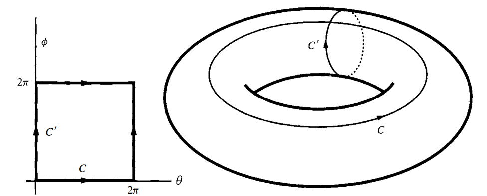
Example. Let’s take a look at 2-dimensional torus, sometimes denoted by $\mathbb{T}^2$. In the figure below two closed curves are shown, $C$ and $C’$, but non of them are the boundary of any surface. On way to see it is that non of the $C$ and $C’$ can be shrunk to a point without leaving the torus. Thus, we don’t expect every closed form to be exact. For instance, consider two forms $d\theta$ and $d\phi$, where $\theta$ parametrized $C$ and $\phi$ parameterize $C’$, they are closed but not exact, for
\[\oint_{C}d\theta=2\pi\neq 0\]which can only be true if $d\theta$ is not exact. The same goes for $d\phi$.
For historical reasons, that fact that $dd=0$ is called the Poincare’s lemma (not Poincare’s Theorem), even though Poincare utilized this result before the invention of exterior calculus! There is a partial converse to this result, practically says that the converse to Poincare lemma is locally true.
Theorem. For a closed differential form with degree no less than $1$, namely $\beta\in\Omega^p(M)$ and $p\geq {1}$, then there exists a neighborhood $U$ of $x\in M$ and a $(p-1)$-form $\alpha\in\Omega^{p-1}(M)$ such that $\beta =d\alpha$.
Proof. It’s enough to consider $R^n$ instead of $M^n$ since on a small-enough neighborhood $U_{x}$, there is always an diffeomorphism between $U_{x}$ and $R^n$, denoted by
\[\phi:U_{x}\to B^n\]where $B^n$ is a $n$-dimensional open ball in $R^n$.
Since $\phi$ is diffeomorphic, $\phi^{-1}$ exists. Then we can use $\phi^{-1}$ to pull back a closed p-form $\beta\in\Omega^p(M)$ from $M$ to $R^n$. $(\phi^{-1})^\ast \beta$ is also closed, since pullback and $d$ commute with each other. So we just need to find the potential for $(\phi^{-1})^\ast \beta$, call it $\alpha$, then $\phi^\ast\alpha$ is the potential we are looking for.
We may assume the $\beta$ is a closed $p$-form on an open ball $U$ of $\mathbb{R}^n$. Consider the deformation
\[\phi_{t}: \mathbf{x} \to(1-t)\mathbf{x}\]with velocity
\[\mathbf{v}(t,\mathbf{y}) = \frac{d}{dt} \mathbf{y}(t) = -\mathbf{y}(t=0) = - \frac{\mathbf{y}}{(1-t)}\]for $t\neq 1$. Note that $\phi_{0}$ is the identity map that maps a point in $\mathbb{R}^n$ to itself, thus $\phi_{0}^\ast$ is the identity pullback map that maps a differential form to itself, similarly $\phi_{1}^\ast$ is the zero map.
By introducing parameter $t$ we have effectively extended the “spatial” manifold $\mathbb{R}^n$ to the “spacetime” manifold $\mathbb{R}^{n+1}$, a time dependent tensor field in $\mathbb{R}^n$ can be regarded as a tensor field in spacetime.
Considering $\beta = \beta(\mathbf{x})$ as a time-independent $p$-form on $\mathbb{R}^n$, we have
\[\beta(\mathbf{x}) = \phi_{0}^\ast \beta(\mathbf{x}) = \phi_{0}^\ast \beta(\mathbf{x})-\phi_{1}^\ast \beta(\mathbf{\phi_{1}x}) = \int_{1}^{0} ds \, \frac{d}{ds} \phi_{s}^\ast \beta(\mathbf{\phi_{s}x}) .\]Using
\[\frac{ \partial }{ \partial t } \phi_{t}^\ast \alpha = \phi_{t}^\ast \left\{ \frac{ \partial \alpha }{ \partial t } + i_{\mathbf{v}} d\alpha + d i_{\mathbf{v}}\alpha \right\}\]where $\mathbf{v}=\partial\phi_{t}(x) / \partial t$ is the velocity field. Together with $d\beta=0$ and $\partial\beta / \partial t=0$, Eq. (1) becomes
\[\beta(\mathbf{x}) = \int_{1}^{0} ds \, \phi_{s}^\ast d[i_{\mathbf{v}(\phi_{s}\mathbf{x})}\beta(\phi_{s}(\mathbf{x}))] = d \int_{1}^{0} ds \, \phi_{s}^\ast [i_{\mathbf{v}(\phi_{s}\mathbf{x})}\beta(\phi_{s}(\mathbf{x}))]\]where we first exchanged $d$ and $\phi_{s}^\ast$ then moved $d$ outside of the integral sign, which is allowed since the integral domain is unchanged. Thus
\[\beta = d\alpha,\quad \alpha = \int_{1}^{0} ds \, \phi_{s}^\ast [i_{\mathbf{v}(\phi_{s}\mathbf{x})}\beta(\phi_{s}(\mathbf{x}))]\]Note that the proof stands because for every point in $\mathbb{R}^n$ is associated a neighborhood that can be contracted to the point; that is, there is a deformation given by $\mathbf{x}\mapsto(1-t)\mathbf{x}$ that collapses the neighborhood to the point.
Let us now write down the expression for $\alpha$ in detail. Let $\mathbf{y}:=\phi_{s}(\mathbf{x})=(1-t)\mathbf{x}$, then
\[i_{\mathbf{v}(\phi_{s}\mathbf{x})}\beta(s,\mathbf{y}) = i_{\mathbf{v}(\mathbf{y})}\beta(s,\mathbf{y}) = v^j(\mathbf{y})\beta_{jK}(\mathbf{y})dy^K = -\frac{y^i}{1-s}b_{jK}(\mathbf{y})dy^K\]where we require the indices in $K$ increases monotonically, this saves as the annoying factors like ${1} / {n!}$.
To take $\phi_{s}^\ast$ of this (p-1)-form is to change the coordinates from ${y}$ to $\left{ x \right}$. Putting $\tau=1-s$ we have
\[\alpha = \int_{0}^{1} d\tau \, \tau^{p-1}x^jb_{jK}(\tau \mathbf{x})dx^K\]where the increasing order in the index set $K$ is understood.
Since all of $\mathbb{R}^n$ can be contracted to a point, the conclusion holds for $\mathbb{R}^n$ globally. If $\beta$ is closed in $\mathbb{R}^n$, then it is also globally exact.
Corollary. If $\text{div } \mathbf{B} = 0$ in $\mathbb{R}^3$ then $\mathbf{B}= \text{curl }\mathbf{A}$ for some $\mathbf{A}$.
Find Potentials
Consider the electric field due to a charge $q$ at the origin. In spherical coordinates
\[\mathbf{E}=\frac{q}{r^{2}}\partial_{r}\]for $r>0$. Using the Euclidean metric in spherical coordinates,
\[ds^{2} = dr^{2}+r^{2}(d\theta^{2}+\sin ^{2}\theta d\phi^{2})\]we find
\[\mathcal{E}=\mathbf{d}(-q / r),\quad \mathbf{d} = dx\wedge \partial_{x}+dy\wedge \partial_{y}+dz\wedge \partial_{z}\]where $\mathcal{E}:=E_{i}dx^i$ is the electric field intensity 1-form, and $q / r$ is the familiar scalar potential.
Enjoy Reading This Article?
Here are some more articles you might like to read next: