Betti Numbers
Disclaimer: Nothing in this note is original.
The lack of simple connectivity is but one measure of topological complexity for a space. The Betti number is another.
Singular Chains and Their Boundaries
First we introduce the geometric building block, the standard p-simplex, or sometimes called the Euclidean p-simplex. It is the convex set $\Delta_ {p} \subset \mathbb{R}^{p}$ generated by the $p+1$ points,
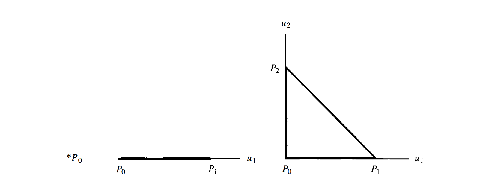
We shall write
\[\Delta_ {p} = (p_ {0}, \dots, p_ {p}).\]In barycentric coordinates, we can write
\[\Delta_ {p} = \left\{ (a_ {0}p_ {0} + \dots + a_ {p} p_ {p}) \,\middle\vert\, \sum a_ {i}=1 \text{ and } a_ {i}>0 \right\}.\]Simplex is a generalization of the notion of a triangle to arbitrary dimension. It is so-named because it represents the simplest possible polytope ( a geometric object with flat sides) in any given dimension.
A singular p-simplex is something defined in a given manifold, no longer in $\mathbb{R}^{p}$. It is a differentiable map
of a standard p-simplex into M. We shall use $\sigma_ {p}$ to denote both the map itself and the image of the map.
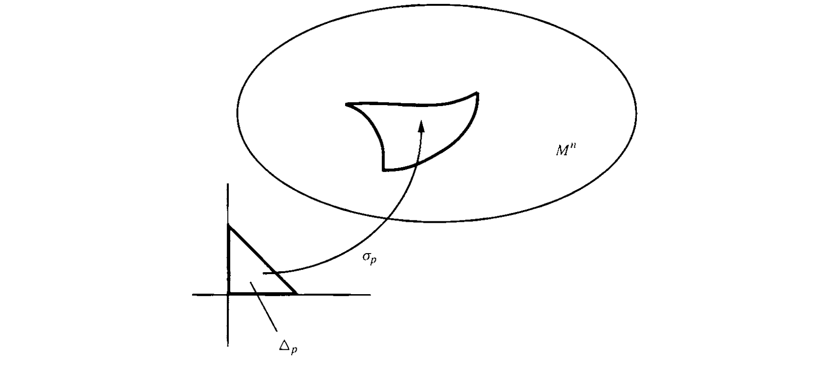
Note that singular simplexes are the natural object over which one integrates p-forms of M via the pull-back
\[\boxed{ \int _ {\sigma} \, \alpha^{p} := \int _ {\Delta} \, \sigma ^\ast \alpha^{p}. }\]We emphasis that there is no restriction on the map $\sigma_ {p}$, for example, the image of it could very well be a point, we don’t care. It is possible because there is no restriction on the maps we use for pull-backs. Maybe that’s why it is called singular simplex, because the image can be singular.
We will talk about the surface of p-simplexes, thus we need to introduce the concept face. First let us define faces for the standard simplexes. The $k$-th face $\Delta_ {p-1}^{(k)}$ of $\Delta_ {p}$ is something one dimension less:
where the hatted vertex is supposed to be deleted. We could say the the k-th face is the face opposite the vertex $p_ {k}$. Note that, restrictively speaking, the k-th face is not itself a standard simplex for it is a $p-1$ dimensional object in $p$ dimensional space; instead, we consider it as a singular simplex in $\mathbb{R}^{p}$, given by the map
\[f_ {k} : \Delta_ {p-1} \to \Delta_ {p}.\]To be mathematically accurate, $f_ {k}$ is the unique affine map (i.e., a linear map followed by a translation of origin) of $\mathbb{R}^{p-1}$ into $\mathbb{R}^{p}$ that sends $p_ {0}\to p_ {0},\dots, p_ {k-1}\to p_ {k-1},p_ {k}\to p_ {k+1},\dots,p_ {p-1}\to p_ {p}$, namely we jumped the $k$-th point in $\mathbb{R}_ {P-1}$. But this is just making things more complicated.
The composition of maps naturally gives us the composition of the construction of singular simplexes. Let $\sigma$ be a singular simplex in $M$ and a map $\phi: M \to V$, then $\phi\;\circ\;\sigma$ defines a singular simplex in $V$. In particular $\sigma \;\circ\;f_ {k}: \Delta_ {p-1}\to M$ defines a singular simplecial face in $M$.
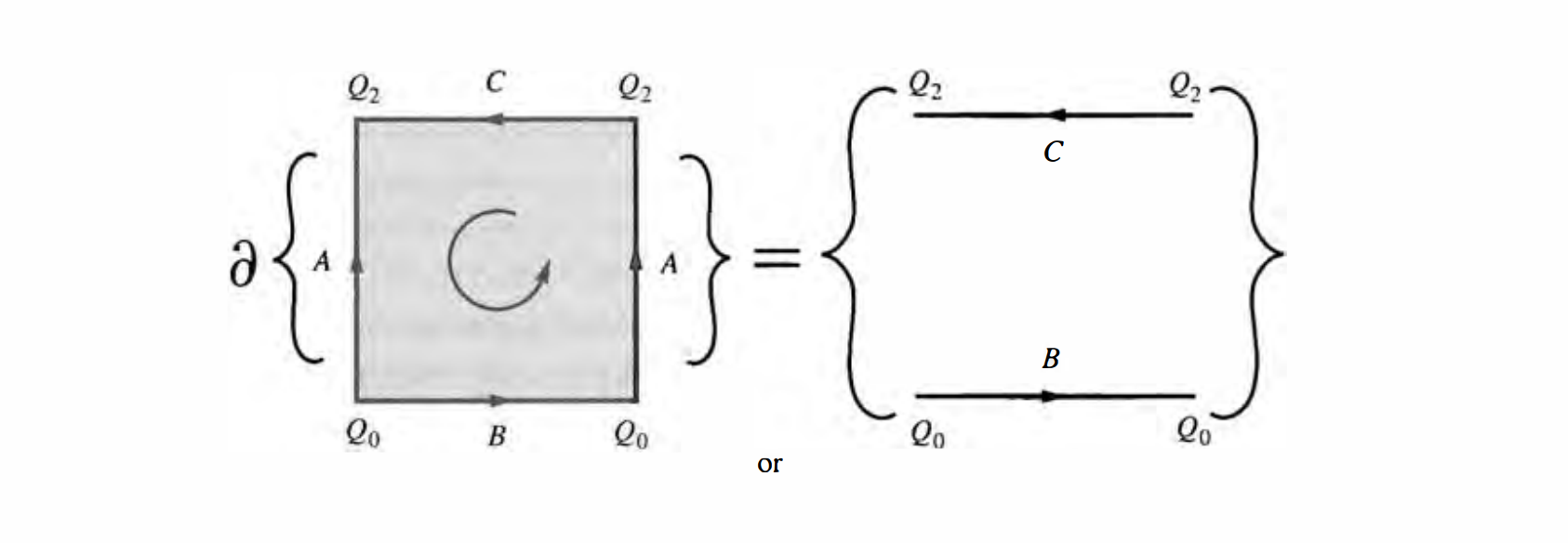
Given the image of a simplex we can easily read off the boundary of it. In algebraic topology, we want to study such intuitive, geometric operations using algebraic method, thus we want to find a algebraic operator that gives us the boundary of a simplex. In this spirit, we define the boundary $\partial\Delta_ {p}$ of the standard p-simplex, to be the formal sum (formal means we don’t ask the meaning about the result of the summation, just regard summation as a formal operation, in this sense we are allow to add one apple to one square) of singular simplexes,
\[\partial \Delta_ {p} = \partial (p_ {0},\dots,p_ {p}) := \sum_ {k}(-1)^{k} (p_ {0},\dots,\widehat{p_ {k}}, \dots,p_ {p}) = \sum_ {k}(-1)^{k} \Delta_ {p-1}^{(k)}\]whereas for the $0$-simplex we put $\partial\Delta_ {0}=0$.
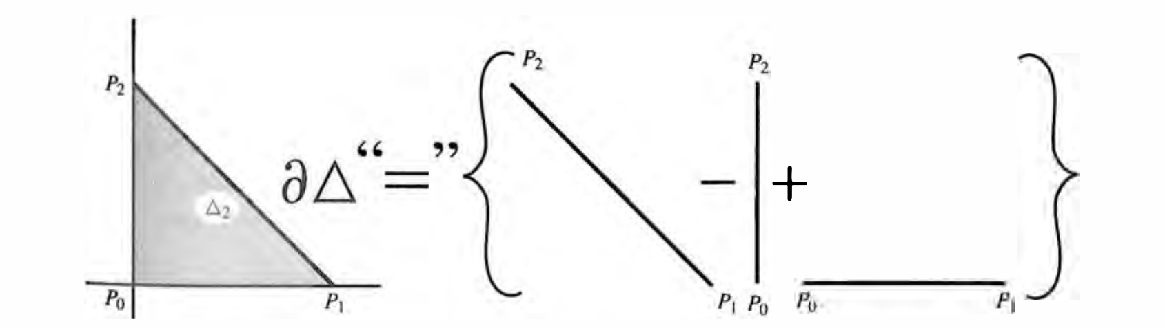
$\Delta_ {2}$ is an ordered simplex, that is, it is ordered by the given order of its vertices. From this ordering we may extract an orientation. The ordering is defined to be given by $\mathbf{e}_ {1} = (p_ {1}p_ {1}) = p_ {0} -p_ {1}$ and $\mathbf{e}_ {2}=(p_ {0}p_ {2}) = p_ {2}-p_ {0}$. We think of the minus sign in front of $(p_ {0}p_ {2})$ as effectively reversing the orientation of this simplex. It should come naturally. We define the orientation of the boundary in this way such that the Stoke’s theorem for a 1-form $\alpha$ in the plane can be express in the neat form:
If we write the integral in a different form, define some kind of a “inner product” between a differential form and a simplex on which it integrate,
\[\left\langle \Delta, \omega \right\rangle := \int _ {\Delta} \, \omega\]then Eq. (1) can be written as
\[\left\langle \partial \Delta , \alpha \right\rangle = \left\langle \Delta,d\alpha \right\rangle,\]and we may say that $\partial$ is the dual operation to $d$.
The boundary of a simplex is itself not a simplex, since it is a formal sum of simplexes. It is an example of a new type of object, an integer chain. To be specif, the boundary $\partial\Delta_ {p}$ is an integer $(p-1)$-chain. For topological purposes it is necessary, and no more difficult, to allow much more general coefficients than merely $\pm 1$, or integer in that sense. Let $G$ be any abelian, that is, commutative, group. The main groups of interest to us are
- $G=\mathbb{Z}$, the group of integers.
- $G=\mathbb{R}$, the additive group of real numbers.
- $G=\mathbb{Z}_ {2} = \mathbb{Z} / 2 \mathbb{Z}$, the group of integers mod 2.
The notation $\mathbb{Z} / 2 \mathbb{Z}$ means that in the group $\mathbb{Z}$ of integers we shall identify any two integers that differ by an even integer, that is, an element of the subgroup $2\mathbb{Z}$. The elements of $2\mathbb{Z}$ are two equivalent classes in $\mathbb{Z}$, namely $[0]$ and $[1]$, where it is conventional to use square brackets to denote the equivalent class.
We define a (singular) p-chain on $M$, with coefficients in the abelian group $G$, to be a finite formal sum
This formal definition means the following. The p-chain can be considered as a function defined on all the singular complexes, whose value at $\sigma_ {p}^{i}$ is $g_ {i}$. So a p-chain is a function
\[p-\text{chain } : \text{ singular complexes} \to G.\]It has the property that its value is zero for all but finite simplexes.
We add two p-chains by simply adding the functions, namely adding the coefficients for same simplexes.
The collection of all singular p-chains of $M$ with coefficients in $G$ themselves form an abelian group, the singular p-chain group of $M$ with coefficients in $G$, written
A chain with integer coefficients will be called simply an integer chain.
For example, we can talk about the group of chains of standard simplexes, denoted $C_ {p}(\mathbb{R}^{p};\mathbb{Z})$.
Recall that a homomorphism of an abelian group $G$ into another abelian group $H$ is a map that preserves the addition. Let
be a map, we have already seen that if $\sigma$ is a singular simplex of $F$ then the composition $F \;\circ\; \sigma$ is a singular simplex of $V$. We extend $F_ {\ast}$ to be a homomorphism, called the induced chain homomorphism, we just push everything on $M$ to $V$. There is nothing much to say about it.
A natural question to ask is, given a chain, what is its boundary? One might guess, the boundary should be another chain with one less dimension. It turns out to be correct. Starting from the simplest situation, a single complex. If $\sigma: \Delta \to M$ is a singular simplex on $M$, its boundary $\partial\sigma$ is a $(p-1)$-chain defined as follows. Recall that $\partial\Delta_ {p}$ is the $(p-1)$ integer chain
\[\partial \Delta = \sum_ {k} (-1)^{k}\Delta^{(k)}_ {p-1},\]we then define
\[\partial \sigma:= \sigma_ {\ast } \partial \Delta_ {p} = \sum_ {k} (-1)^{k}\sigma_ {\ast }\Delta^{(k)}_ {p-1} = \sum_ {k}(-1)^{k} \sigma^{(k)}_ {p-1}.\]Roughly speaking, the boundary of the image of $\Delta$ is the image of the boundary of $\Delta$! Taking boundary and map are two commutative operations.
Finally, we define the boundary of any singular p-chain with coefficients in $G$ by
\[\partial \sum_ {r} g_ {r} \sigma^{r}_ {p} = \sum_ {r} g_ {r} \partial \sigma^{r}_ {p}.\]How else can you define it?
By construction we then have the boundary homomorphism \(\partial : C_ {p}(M; G) \to C_ {p-1}(M; G).\)
The following statement combines algebra and geometric intuition perfectly. The boundary of a boundary is zero! That is,
Theorem.
\[\partial ^{2} = \partial \;\circ\;\partial =0.\]Interested readers can try to prove it by yourself.
Some 2-Dimensional Examples.
The cylinder Cyl is the familiar rectangular band with the two vertical edges brought together by bending and then sewn together. We wish to exhibit a specific integer 2-chain on Cyl. On the right we have the rectangular band and we have labeled six vertices. The labels on the two vertical edges are the same, since the band is to be bent and the two edges are to be sewn.
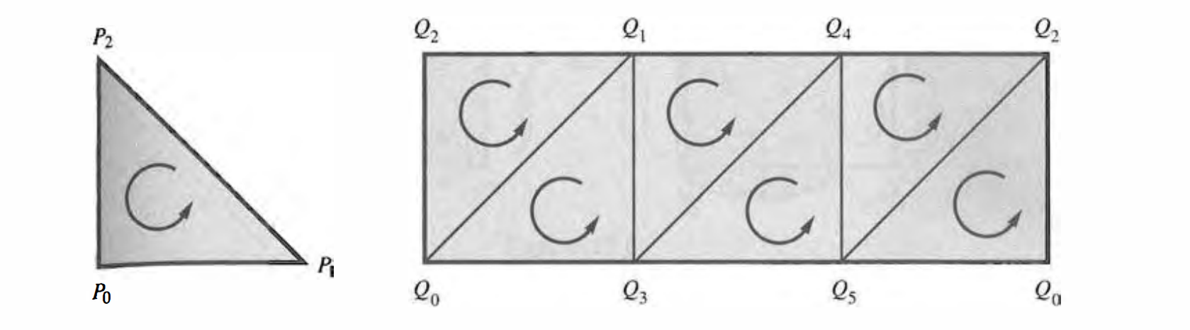
On the band we have indicated six singular (ordered) 2-simplexes. We shall always write a singular simplex with vertices in increasing order. For example, the singular simplex $(Q_ {1}Q_ {3}Q_ {4})$ is the image of a map of $(P_ {0} P_ {1} P_ {2})$ to the band. After the band is bent and sewn we shall then have a singular 2-simplex on Cyl that we shall again call $(Q_ {1}Q_ {3}Q_ {4})$. We have thus broken Cyl up into 2-simplexes, and we have used enough simplexes so that any 1- or 2-simplex is uniquely determined by its vertices.
Regard the whole band as a 2-chain, where the simplex carries the orientation indicated in the figure. Since we always write a simplex with increasing order to its vertices, we put
\[c_ {2}=(Q_ {0}Q_ {1}Q_ {2})-(Q_ {0}Q_ {1}Q_ {3})+\dots\]Then we can write down the expression for the boundary of the “triangulation” of Cyl. It is tedious but straightforward.
It can be shown that the boundary is made of the top edge and bottom edge, with reversed directions.
The next example would be the famous Mobius strip, however we will leave it as a home work. Note that, due to the non-orientable nature of the Mobius band, the property of its boundary will be rather strange.
The Singular Homology Groups
In this section we will answer questions like what is a cycle and Betti number.
The coefficient field
Recall that the boundary of the boundary is zero, $\partial\;\circ\;\partial=0$, which reminds us of the exterior differential which also satisfies $d\;\circ\;d=0$. Turns out their similarity is far more than just that.
An abelian group $G$ is a field, if, roughly speaking, $G$ has not only an additive structure but an abelian multiplicative one also, with multiplicative identity element $\mathbb{1}$ , and this multiplicative structure is such that each $g\neq {0}$ in $G$ has a multiplicative inverse $g^{-1}$ such that $g g^{-1}=\mathbb{1}$. We further demand that multiplication is distributive with respect to addition. The most familiar example is the field $\mathbb{R}$ of real numbers. The ring of inters $\mathbb{Z}$ is not a field, but $\mathbb{Z}_ {p}$ where $p$ is a prime number does form a field.
Given a chain with coefficient group $G$, when $G$ is also a field, denoted $K$, called the coefficient field, then the chain group $C_ {p}(M;K)$ becomes a vector space. Vector spaces are studied to death, we are happy to see an old friend. The scalars in the vector space is given by the coefficient field, and the basis are the singular simplexes. For each scalar $r\in K$ and chain $c=\sum g_ {i} \sigma^{i}$ where $\sigma^{i}$ are singular simplexes, the scalar multiplication is defined in the obvious way,
For the simplicity of the notations, we sometimes omit the subscript that denotes the dimension of the simplices, when there is no confusion introduced. For example $\sigma_ {p}^{i}$ will just be written as $\sigma^{i}$. When we are dealing with a specific space $M^{n}$ and also a specific coefficient group $G$, we shall frequently omit $M$ and $G$ in the notation for the chain group. Then $C_ {p}(M;G)$ becomes just $C_ {p}$.
The vector space of $p$-chains is infinite dimensional since no finite nontrivial linear combination of distinct singular simplexes is ever the trivial $p$-chain $0$.
What about the boundary operation when the coefficients form a field? It becomes a linear transformation! We sometimes write
\[\partial : C_ {p} \to C_ {p-1}.\]Finite simplicial complexes
There is a related notion of simplicial complex with its associated simplicial (rather than singular) chains. Consider the Mobius band for example, we can introduce the triangulation of the Mobius band, by covering it with 2-simplexes. If you have done it, you’ll see that, just like for the cylinder, we need six 2-simplexes at least to triangulate it. These 2-simplexes are not just any singular simplexes, they are isomorphic to the standard 2-simplex. Suppose now that instead of looking at all singular simplexes on Mobius we only allow these six 2-simplexes and allow only 1-simplexes that are edges of these 2-simplexes, and only the six 0-simplexes (i.e., vertices) that are indicated. We insist that all chains must be combinations of only these simplexes; these form the “simplicial” chain groups $\overline{C}_ {p}, p =0,1,2$. $\overline{C}_\ast(\text{Mobius};G)$ is a group with the following generators which are singular complexes.
- Six vertices, the 0-simplexes;
- Twelve edges, the 1-simplexes;
- Six faces, the 2-simplexes. They all fit together
nicelyto form the triangulation of the Mobius band. If we have a field $K$ for coefficients, then we have a vector space generated by these singular complexes. They are finite dimensional vector space. Even better, the boundary operator is closed in the simplicial complex! We have
In other words, in a simplicial complex, we are given some geometric object and its triangulation, like the triangulation of the Mobius in the previous example. Then the simplicial complex is the chain group form by the singular simplexes. The boundary operation is closed in the chain. It is like the minimal working environment for leaning the algebraic topology of some manifold.
Return to the general case of singular chains with a coefficient group $G$. First we will make some really abstract definitions, then coming backing to concrete examples later.
We define a (singular) p-cycle whose boundary is zero. The collection of all the p-cycles are denoted by $Z$,
That is, the kernel $\partial^{-1}(0)$ of the group homomorphism $\partial$, which by the group property is also a group, called the p-cycle group.
We define a p-boundary $\beta_ {p}$ to be the boundary of some $(p+1)$-chain. The collection of all such chains are the image (range) of the group homomorphism $\partial$, which also forms a group.
To summarize, we have defined
- The group of p-chains $C_ {p}$;
- The cycle group of p-cycles $Z_ {p}$;
- The boundary group of p-boundaries, $B_ {p}$.
Of course if the coefficients are also fields then instead of group we would have a vector space.
Next, let us consider the integral of p-forms on the p-chains, which are p-dimensional manifolds. Given a p-chain $c_ {p} = \sum b_ {i} \sigma^{i}$, it is natural to define the integral to be the linear combination of the integrals on individual. Given some p-form $\alpha$, we define
\[\int _ {c_ {p}} \, \alpha := \sum_ {i} b_ {i} \int _ {\sigma^{i}} \, \alpha.\]Then the duality between $\partial$ and $d$ tells us that
\[\int _ {c_ {p}} \, d\alpha^{p-1} = \int _ {\partial c_ {p}} \, \alpha^{p-1}=\sum_ {i} b_ {i} \int _ {\partial \sigma^{i}} \, \alpha^{p-1}.\]Furthermore, if $\alpha$ is closed, $d\alpha=0$, then we can change the integral manifold by a filled submanifold without changing the integral value. To be accurate, if $z_ {p}$ and $z’_ {p}$ are two cycles (note, not just any chain), and they differ by a boundary,
\[z_ {p} - z'_ {p} = \partial c_ {p+1}=: b,\]we have
\[\int _ {z} \, \alpha-\int _ {z'} \, \alpha = \int _ {b} \, \alpha = \int _ {\partial c_ {p+1}} \, \alpha = \int _ {c_ {p+1}} \, d\alpha =0.\]Thus, as far as closed forms go, boundaries contribute nothing to integrals. When integrating closed forms, we may identify two cycles if they differ by a boundary. This identification turns out to be important also for cycles with general coefficients.
If $G$ is an abelian group and $H$ is a subgroup, let us define two elements $g$ and $g’$ of $G$ are equivalent if they differ by some element of $H$,
\[g \sim g' \text{ iff } g-g' \in H\]Note that it does not matter where $H$ acts on $g’$ from left or right since we assume the group is abelian, hence the use of minus sign, instead of division. Sometimes we say $g\sim G’ \text{ mod }H$, the set of equivalent classes is denoted $G / H$, read $G$ mod $H$. If $g\in G$ we denote the equivalence class of $g$ in $G / H$ by $[g]$, or sometimes $g+H$. Such an equivalent class is called coset, and $g$ is called the representative of $[g]$. Of course any element of $[g]$ can be a representative $[g]$. The addition and subtraction of two equivalent classes are defined element-wise. In this way, we make $G / H$ into a group, called the quotient group. This is exactly the procedure we followed when constructing the group $\mathbb{Z}_ {2} = \mathbb{Z} / 2\mathbb{Z}$, integer mod 2.
We always have a map $\pi: G\to G / H$ that assigns to each $g$ its equivalence class $[g]$. $\pi$ is, by construction, a homomorphism.
When $G$ is a vector space $E$, and $H$ is a subspace $F$, then $E / F$ is again a vector space. If $E$ is further an inner product space, then $E / F$ can be identified with the orthogonal complement of $F$. If $E$ does not carry a specific inner product, then there is no natural way to identify $E / F$ as a subspace of $E$.
Return now to our singular cycles. We say that two cycles $z$ and $z’$ in $Z_ {p}(M;G)$ are equivalent or homologous, if they differ by a boundary. In the case of the cycles $Z_ {p}$ and boundaries $B_ {p}$, the quotient group is called the $p$-th homology group, written $H_ {p}(M;G)$
When $G=K$ is a field, the cycles, boundaries and chains become vector spaces. Otherwise they are module.
We have seen that the group of cycles and boundaries are infinite dimensional, but their quotient is usually finite dimensional! It can be shown that this is a case if $M$ is compact. Before going into details we mention a purely algebraic fact that will be useful.
Theorem. Let $\phi: G_ {1}\to G_ {2}$ be a homomorphism between two abelian groups. $\phi$ also maps the subgroup $H_ {1}<G_ {1}$ to the subgroup $H_ {2}<G_ {2}$. Then $\phi$ induced a homomorphism $\phi_ {\ast}$ between the two quotient groups
\[\phi_ {\ast } : G_ {1} / H_ {1} \to G_ {2} / H_ {2}.\]We will omit the proof.
We then have the following topological situation. If $M$ is a compact manifold, there is a triangulation of $M$ by a finite number of $n$-simplexes each of which is diffeomorphic to the standard $n$-simplex. This means that $M$ is a union of such $n$-simplexes and any pair of such simplexes either are disjoint or meet in a common r-subsimplex (vertex, edge, etc. ) of each. For example, think of the triangulation of a cylinder. These simplexes can be used to form a simplicial complex, denoted with a bar, we have $\overline{Z},\overline{B}$ and $\overline{C}$. The advantage of simplicial complex is that as a group, they are finitely generated. Now, any simplicial cycle can be considered a singular cycle, since we have a trivial homomorphism from $\overline{Z}$ to $Z$. Elements in $\overline{B}$ are also elements in $B$. Thus we have an induced homomorphism of the simplicial homology class $\overline{H}$ to the singular homology class $H$. It is then a nontrivial fact that for compact manifolds $H = \overline{H}$, that is, the $p$-th singular homology group is isomorphic to the $p$-th simplicial homology group! Recall that a homomorphism is an isomorphism if it is one-to-one and onto. In particular the singular homology groups are also finitely generated (even though the singular cycles clearly aren’t).
When $G$ is the field of real numbers, $G=\mathbb{R}$, the dimension of the vector space $H_ {p}$ is called the $p$-th Betti number, written $b_ {p} =b_ {p}(M)$
In words, $b_ {p}$ is the maximal number of $p$-cycles on $M$, their real linear combination can never be a boundary.
Let $F : M\to V$ be a map. Since $F_ {\ast}$ commutes with the boundary $\partial$, we know that $F_ {\ast}$ takes cycles into cycles and boundaries into boundaries. Thus $F_ {\ast}$ sends homology classes into homology classes, and we have an induced homomorphism
\[F_ {\ast }: H(M;G) \to H(V;G).\]Thanks to this property, homeomorphic manifolds have isomorphic homology groups. We say that the homology groups are topological invariants.
Homology Groups of Familiar Manifolds
Any point $p\in M$ is a 0-chain, and by definition $\partial\; 0\text{-chain}=0$.
A smooth map $C:[0,1]\to M$ is a curve, which is a compact, singular 1-chain. It is compact since $[0,1]$ is compact in $\mathbb{R}$ and the continuous map of any compact manifold is itself compact. The boundary of $C$ is $C(1)-C(0)$.
Intuitively, a piecewise continuous curve can be glued together by pieces of smooth curves. It is again a 1-chain.
A manifold $M^{n}$ is said to be (path-)connected if any two points $p$ and $q$ can be joined by a piecewise smooth curve $C$. The next statement may take some time to get: any two 0-simplexes with the same coefficient, in a connected manifold, are homologous. In the case of $p$ and $q$, we have $p-q$ is the curve connecting $q$ to $p$, but the curve itself is a 1-chain, thus $p-q$ is the boundary of this 1-chain, call it $C$. Then $p = q + \partial C$. Thus $p,q$ are homologous. Roughly speaking, two manifolds differ by a stuffed manifold are homologous. Also, since the boundary of a 1-chain is always make of more than one (even number of) points, a single point is not the boundary of anything. Thus any particular point $p$ of a connected space defines a 0-cycle that is not a boundary, and any 0-chain is homologous to a multiple $gp$ of $p$. We have
For example, $H_ {0}(M;\mathbb{Z})$ is the set ${ 0,\pm 1 p, \pm 2p, \dots }$, it doesn’t matter which $p$ we choose since they are all homologous to each other. Another example, $H_ {0}(G,\mathbb{R})$ is the 1-dimensional vector space consisting of all real multiples of the “vector” $p$, this vector space is isomorphic to $\mathbb{R}$ since there are only one basis, we usually write
\[H_ {0}(M;\mathbb{R}) =\mathbb{R}.\]In particular, a connected manifold has Betti number $b_ {0}=1$. Similarly, if $M$ is not connected but consists of $k$ connected sub-manifold then the Betti number is $b_ {0}=k$, the homology group is
\[H_0(M;\mathbb{R}) = \mathbb{R} \,\oplus\, \mathbb{R} \,\oplus\, \dots\mathbb{R} = \mathbb{R}^{k}.\]We should mention that in topology there is the notion of a connected space; M is connected if it cannot be written as the union of a pair of disjoint open sets. This is a weaker notion than path-wise connected, but for manifolds the two definitions agree.
Next, consider a compact p-dimensional manifold $V$ with no boundary. By triangulating $V$ one may show that $V$ always defines an integer $p$-cycle, $V$ itself. It is denoted by $[V]$. On the other hand, consider a non-orientable manifold, like a Klein bottle. The Klein bottle can’t be embedded in $\mathbb{R}^{3}$ but we can exhibit an immersion with self-intersection. This is the surface obtained from a cylinder when the two boundary edges are sewn together after one of the edges is pushed through the cylinder. Then, given a triangulation, we see that the boundary is not vanishing anymore, $[\text{Klein bottle}]$ is not a cycle, even though the manifold has no boundary!
The above considerations lead us to the following theorem.
Theorem. Every closed oriented p-dimensional manifold $V\subset M^{n}$ defines a $p$-cycle $g[V]$ in $H_ {p}(M;G)$, by associating the same $g\in G$ to each oriented p-triangle in a suitable triangulation of $V$.
Thus a p-cycle is a generalization of a p-dimensional closed orientable manifold.
Rene Thom has proven the following theorem.
Thom’s Theorem. Every real $p$-cycle in $\mathbb{M}^{n}$ is homologous to a finite formal sum of closed oriented submanifolds with real coefficients.
One useful computational tool is concerned with deformations. We can deform a p-manifold, or a p-chain, just like how we would deform a curve. We shall not go to the details but merely mention the following theorem.
Deformation Theorem. If a cycle $z$ is deformed to $z’$ then $z’$ is homologous to $z$. Their difference is the boundary of something.
This follows from the fact the process of deformation sweeps out a stuffed sub manifold.
Finally, we mention that
\[H_ {p}(M^{n};G)=0 \text{ for } p >n.\]Some examples
Let’s consider the n-dimensional sphere $\mathbb{S}^{n}$. We have
\[H_ {0}(\mathbb{S}^{n};G)=G\]since $\mathbb{S}^{n}$ is compact and connected. $z_ {p}, 0<p<n$ is some singular p-chain, it is homologous to some p-chain in the simplicial complex of the sphere with certain triangulation. The usual triangulation of the sphere results from inscribing an $(n+ 1 )$-dimensional tetrahedron and projecting the faces outward from the origin until they meet the sphere. Since a general $z_ {p}$ for $p<n$ can be contracted to a point, which is only nontrivial in $H_ {0}$, we have
\[H_ {p}(\mathbb{S}^{n};G) = 0, \quad p\neq 0 \text{ and }n.\]If $p=n$ we have shown that $[\mathbb{S}]$ itself is a cycle but not a boundary of anything else, since there is nothing of $n+1$ dimension, thus
\[H_ {n}(\mathbb{S}^{n};G)=G.\]For the 2-torus, $\mathbb{T}^{2}$, we have $H_ {0} = H_ {2}=G$. We state the result here only, interested readers can refer to, e.g., Nakaraha:
\[H_ {1}(\mathbb{T}^{2},G) = G \otimes G.\]As our last example, consider the real projective plane $\mathbb{R}P^{2}$. The model is the 2-disc with antipodal identifications on the boundary circle. The upper and lower semicircles arc are the same closed curve. Take the coefficient group to be the integers. We have
\[H_ {0}(\mathbb{R}P^{2};\mathbb{Z}) = \mathbb{Z},\quad H_ {2}(\mathbb{R}P^{2;\mathbb{Z}})=0.\]Any 1-chain can be deformed to the boundary of the projective plane, call it $A$. Another interesting thing about $A$ is that $2A=0$, thus we have
\[H_ {1}(\mathbb{R}P^{2};\mathbb{Z}) = \mathbb{Z}_ {2}.\]Enjoy Reading This Article?
Here are some more articles you might like to read next: