Holonomic and Nonholonomic Constraints
The Frobenius nonholonomic constraints
Given a smooth non-vanishing vector field in $\mathbb{R}^{3}$, one can always find a smooth family of integral curves, that is, a family of curves that are 1) non-intersecting and 2) always tangent to the given vector field.
What about instead of vector field, one is given a family of 2-planes $\Delta$ in $\mathbb{R}^{3}$? At every point, instead a vector, now we have an infinitesimal 2 dimensional plane. Can we always find a family of surfaces, call it the integral surfaces, which are non-intersecting and everywhere tangent to $\Delta$?
Suppose we can. Let $C:t\mapsto x(t)$ be a parametrized curve that is transverse to the family of supposed integral planes everywhere, as shown in the figure below. As can be seen, at each $t$ the curve $C$ is perpendicular to the integral plane. Then, at least locally, we can always define a function $f(\mathbf{x})$ such that its level surfaces are the integral surfaces, that is, the level surface given by $f=t$ consists of the supposed integral surface that is pierced by $C(t)$ at time $t$.
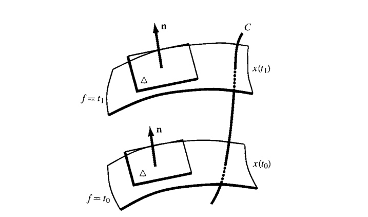
Then the normal vector of the integral domain must be parallel to $\nabla f(\mathbf{x})$. Write $\mathbf{n}=\lambda(x)\nabla f$ for some function $\lambda$. In Cartesian coordinates, there is a simple connection between vector and covector, we can write the normal covector $\nu$ from the normal vector,
\[\nu:= \lambda df = n_{i} dx^{i}.\]The derivative of $\nu$ is
\[d \nu = d(\lambda)\wedge df = \left( \frac{1}{\lambda}d\lambda \right)\wedge (\lambda df)=d\ln \lambda \wedge \nu,\]in short words we have $d\nu=(\text{sth})\wedge\nu$ itself. Then we have Euler’s integrability condition, if such integral plane exists then
\[\boxed{ \nu \wedge d\nu=0,\quad \text{i.e. } \mathbf{n}\cdot \text{curl }\mathbf{n} =0. }\]This condition is a necessary condition for the integral surface to exist.
The trick here is that, when dealing with 2-surfaces, it is usually (I dare not say always) simpler to consider the normal vectors.
As a trivial example, consider the case where $d\nu=0$. Locally we can always find a $\beta$ such that $\nu=d g$, in the language of vectors it would be $\nabla \times \mathbf{v}=0 \implies \mathbf{v}=\nabla g$. The normal vector is perpendicular to the surface $g=\text{const}$.
As a counter example, consider the planes $\Delta$ normal to the vector
\[\mathbf{n} = y\partial_{x}-x\partial_{y} +z\partial_{z}\]where $\partial_{x,y,z}$ are the vector basis. Direct computation shows that
\[d\nu = d(ydx-xdy+zdz) = -2dx\wedge dy,\quad \nu d\nu=-2z dx\wedge dy\wedge dz\neq 0,\]the Euler’s integrability condition is not satisfied, there can’t be integral surfaces.
Consider the normal vector $\mathbf{n} = y\partial_{x}-x\partial_{y} +\partial_{z}$, classically the infinitesimal plane that is orthogonal to this vector at point $(x_{0},y_{0},z_{0})$ is given by the collection of the infinitesimal vectors that are perpendicular to $\mathbf{n}$, define
\[\mathbf{A}=(x-x_{0},y-y_{0},z-z_{0})\equiv (a_{1},a_{2},a_{3}),\]then $\Delta$ is given by the condition
\[\mathbf{A} \cdot \mathbf{n}(x_{0},y_{0},z_{0})=0\]which is sometimes written as
\[ydx-xdy+dz=0\]where $dx,dy,dz$ are now infinitesimal incrementations instead of the basis of differential forms.
Now, let us regard $\nu=ydx-xdy+dz$ as a 1-form.
Definition. The collection of all the planes given by vectors $\mathbf{A}$ such that
\[i_{\mathbf{A}}\nu=0\]is called the distribution associated to the 1-form $\nu$.
This is not to be confused with the generalized functions also called distributions.
In general in $\mathbb{R}^{3}$ one would describe a family of planes by writing
\[\nu=P_{1}dx^{1}+P_{2}dx^{2}+P_{3}dx^{3} = 0\]where $P_{1,2,3}$ are smooth function, thus $\nu$ can be seen as a smooth 1-form field. To find the integral surfaces is to find the solution of the above equation. Such a plane can be parameterized by two variable $s:(u^{1},u^{2})\mapsto\mathbf{x}(u^{1},u^{2})$, the equation becomes
\[\left\langle \nu, \frac{ \partial \mathbf{x} }{ \partial \mathbf{u} } d\mathbf{u} \right\rangle =\nu_{i} \frac{ \partial x^{i} }{ \partial u^{j} } u^{j}=0 \text{ for all }u^{j},\]we can pullback $\nu$ to the ${ u^{I} }$ coordinate system and claim that $s^{\ast}\nu=0$. We have seen that $\nu \wedge d\nu$ is a necessary condition for $s^{\ast}\nu=0$ to have a 1-parameter family of solutions. We will show that it is also a sufficient condition.
Before we go further it is convenient to introduce the definitions of $k$-distribution and $k$-integral manifold,
Definition. A $k$-dimensional distribution $\Delta_{k}$ on $M^{n}$ assigns in a smooth fashion to each $x \in M^{n}$ a $k$-dimensional subspace $\Delta_{k}$ of the tangent space to $M^{n}$. An $r$-dimensional integral manifold of $\Delta_{k}$ is a $r$-dimensional submanifold of $M$ such that it is tangent to $\Delta_{k}$ everywhere. The $k$-distribution $\Delta_{k}$ is said to be (completely) integrable if locally there are coordinates $x^{1},\dots,x^k,y^{1},\dots,y^{n-k}$ for $M$ such that the coordinate slices $y^{1}=\text{const},\dots,y^{n-k}=\text{const}$ are $k$-dimensional integral manifolds of $\Delta_{k}$. Such a coordinate system ${ x,y }$ will be called a Frobenius chart for M.
Roughly speaking, a $k$-dimensional distribution $\Delta_{k}$ is a smooth field of $k$-dimensional subspace of the tangent space.
The fundamental question is, when is $\Delta_{k}$ integrable?
Suppose we are given a distribution $\Delta_{k}$, and a pair of vector fields $X$ and $Y$ such that at every point in an open set $X,Y\in\Delta_{k}$. Suppose $\Delta_{k}$ is integrable, then both $X$ and $Y$ are tangent to the integral manifold, since $\Delta_{k}$ itself is tangent to the integral manifold. Then, some theorem tells us that the Lie bracket $[X,Y]$ is also in the distribution. We can denote this symbolically by
\[\boxed{ [\Delta,\Delta]\subset \Delta. }\]We will see that this condition is also sufficient for showing integrability.
Let $\theta \in\Omega^{1}(x)$ be a non-zero $1$-form at $x$, $\theta$ defines a special vector basis $X$ by $\left\langle \theta,X \right\rangle=1$. All the other vector basis $V$s such that $\left\langle \theta,V \right\rangle=0$ expand a $n-1$ dimensional subspace of $n$-dimensional manifold $M$, called the annihilator or null space of $\theta$ at $x$.
Definition. The null space of $\theta$ at $x$ is expanded by the vectors $V$ such that $\left\langle \theta,V \right\rangle=0$.
Classically one writes $\theta=0$ for this null space. When discussing distributions it is common to call a 1-form $\theta$ a Pfaffian, $\theta=0$ is called the Pfaffian equation.
Let $\theta_{1},\dots,\theta_{r}$ be $r$ linear independent $1$-forms at each point of an open subset of $M$, being linear independent means that $\theta_{1}\wedge\dots \wedge\theta_{r}\neq {0}$. The second you see “open subset” you should realized that we are talking about local properties which might not hold globally. Anyway, with given $\theta_{1},\dots,\theta_{r}$, each of them has an associated null space, the intersection of all the null spaces form a $k=n-r$ dimensional vector space, which is also a distribution since it is smooth, which follows from the smoothness of the $1$-forms. Call this distribution $\Delta_{k}$ as before, we have
\[X\in \Delta_{k} \quad\text{ iff }\quad \theta_{1}(X) = \theta_{2}(X) = \dots=0.\]We may again write this distribution as $\theta_{1}=\dots=\theta_{r}=0$. Note that we do not claim that every distribution can be globally defined by $r$ Pfaffians.
Definition. If the distribution $\Delta$ is closed under Lie brackets, $[\Delta,\Delta]\subset\Delta$, then $\Delta$ is said to be in involution.
We state without proof that, if a distribution is integrable, then it is in involution.
It is interesting that since 2020 involution has taken Chinese media by storm, especially among younger people. Translated as “内卷”, it implies the growing feeling that the struggle to succeed is futile in conditions of economic precarity and structural unfairness. But for a distribution in our note, being in involution is surely a good thing.
If $\Delta_{k}$ is in convolution, then for any Pfaffian $\theta_{\alpha},\alpha=1,\dots,r$ and any pair of vector fields $X,Y$ in the distribution we have
\[d\theta_{\alpha}(X,Y) = X(\theta_{\alpha}(Y)) - (X\leftrightarrow Y) - \theta_{\alpha}([X,Y])=0.\]We say that if $\Delta$ is in involution, then $d\theta_{\alpha}=0$ when restricted to the distribution, namely, when we allow $d\theta_{\alpha}$ only to be evaluated on vectors of $\Delta$.
Conversely, if $d\theta_{\alpha}=0$ when restricted to $\Delta$, then $[\Delta,\Delta]=\Delta$, namely $\Delta$ is in involution. Interested readers can regard the proof as a homework exercise.
The following statements are equivalent locally.
- $\Delta$ is in involution, that is, $[\Delta,\Delta]=\Delta$.
- The Pfaffians $d\theta_{\alpha}$ are zero when restricted to $\Delta$.
-
There are 1-forms $\lambda_{\alpha \beta}$ such that $d\theta_{\alpha}=\sum_{\beta}\lambda_{\alpha \beta}\wedge\theta_{\beta}$. Recall that for two forms $\alpha,\beta$ the wedge product is defined by \(\alpha\wedge\beta(V_{I_{<}})=\sum_{J_{<},K_{<}}\delta_{I}^{JK}\alpha(V_{J})\beta(V_{K}).\)
- $d\theta_{\alpha}$ is not linear independent of $\theta$s, namely $d\theta_{\alpha} \wedge \theta_{1}\wedge\dots \wedge\theta_{r}=0$.
The proof of the equivalence is left as a homework. They all follow more or less from direct derivation.
In summary, we have shown that in a $n$-dimensional manifold, a $k$-dimensional distribution $\Delta_{k}$ can locally be given in two ways, either by exhibiting $k$ linear independent vector fields $V_{I},I={ 1,\dots,k }$, or by exhibiting $n-r$ linear-independent $1$-forms $\theta_{\alpha}$, sometimes called the Pfaffians, and $\Delta_{k}$ is the unions of the annihilators (null space) of all the $\theta_{\alpha}$s. The system is in involution if
plus, if the system is integrable, it is in involution.
To say $[\Delta,\Delta]\subset \Delta$ is equivalent to say that $d\theta=\sum\lambda_{\alpha \beta}\theta_{\beta}$ for some 1-form $\lambda_{\alpha \beta}$ (note here the subscripts $\alpha,\beta$ are not coordinate indices, but part of the name, $\lambda_{\alpha \beta}$ is not a 2-form but an 1-form), which is equivalent to say that $d\theta_{\alpha}$ is zero mod $\theta_{\alpha}$, written as
\[d\theta_{\alpha}=0 \text{ mod } \theta_{\alpha},\]meaning that $d\theta$ becomes zero if all of the $\theta$s are put to zero.
It turns out that, if the system is in involution, it is also integrable. This statement is more useful to us, since it answers our question of when is a distribution integrable. A sketch of the proof (usually attributed to Frobenius) can be found in Frankel’s textbook. We will not quote the full sketch here but only introduce some main results. But before doing that, we need some definitions.
Definition. A smooth map of manifolds $F:W^{k}\to M^{n}$ is called an immersion, and $F(W)$ called an immersed submanifold, if the induced map
is a one-to-one map, namely $\text{ker }F_{\ast}=0$ at each point of $W$.
Note that immersion is different from embedding. Recall that, $W$ is said to be an embedded submanifold of $M$ if $W$ can be locally described by the common locus of some differentiable functions.
In other words, a map of manifolds is an immersion if it is i) smooth and ii) preserves the rank of the tangent vector space everywhere. For example, if $F_{\ast}$ maps two different vectors to the same vector, then it can not be an immersion. There are examples where some manifold $W$ is an immersion but not embedding, for example, on a torus, consider the distribution defined by $d\phi-kd\theta=0$, where $k$ is an irrational number. For details see page 172 of Frankel.
Finally, we state without proof below the Frobenius theorem.
Frobenius Theorem. If the smooth distribution $\Delta_{k}$ is in involution, namely
then it is complete integrable.
The theorem also tells you how to construct the tangent manifold, which we will not mention here, interested readers can refer to online resources. Just a hint: it uses the flow generated by $X_{i}$s.
Integrability and Constraints
If a distribution $\Delta_{k}$ of manifold $M$ is integrable, then the collection of all the integral manifolds form a foliation(叶状结构) of manifold $M$, each connected integral manifold is called a leaf of the foliation. A leaf that is not properly contained in any other leaf is called a maximal leaf.
Note that the maximal leaf is not necessarily a submanifold of $M$. It is because the leaf, which is a special kind of integral manifold, might have peculiar global structures, for example the maximal leaf mind wind the entire manifold over and over again, circle back close to where it started, things like that, making it impossible for a solution of some differential equation, which is necessary for it to be a submanifold.
Chevalley has proved the following.
Theorem. A maximal leaf of a manifold $M$ is a $1:1$ immersed submanifold; that is to say, there is a $1:1$ immersion map $F:V\to M$ where $V$ is the global realization of the maximal leaf.
Recall that the Frobenius theorem tells us when and how is a distribution totally integrable. Historically, it arose in the study of PDEs. Am important example is the so-called system of Meyer-Lie. In such systems one tries to find functions $y^{\beta}=y^{\beta}(x)$, $\beta=1,\dots,r$ such that
with initial conditions
\[y^{\beta}(x_{0}) = y_{0}^{\beta}.\]Note that $b_{i}^{\beta}$ is a matrix of functions of both $x$ and $y$.
By equating mixed partial derivatives,
\[\frac{ \partial^{2} y^{\beta} }{ \partial x^ix^{j} } = \frac{ \partial^{2} y^{\beta} }{ \partial x^jx^{i} }\]we can find the integrability condition. It is obvious that it is the necessary condition, but non-trivial to show that it is also the sufficient condition. For details see page 173 of Frankel.
Consider a dynamical system, such as the movement of a ball in gravity, but with constrains, for example the ball in $\mathbb{R}^{3}$ could be restricted to move on some 2-dimensional surface. The configuration space is a manifold which we denote by $M$. If the constraint reduce the dimension by $1$, then it can in general be written as a polynomial equation, for example if a ball in $\mathbb{R}^{3}$ is restricted to a unit sphere, then the constraint is given by $F(x,y,z)=x^{2}+y^{2}+z^{2}=1$. This constraint can also be written in terms of differential forms,
\[dF=0 \implies xdx+ydy+zdy=0.\]Here the tradition perspective is to regard $dx,dy,dz$ as infinitesimals, not basis of 1-forms, then the equation says that the infinitesimal displacement in $x,y$ and $z$ direction must satisfy certain relation. Or, equivalently, we could regard $dx,dy,dz$ as basis of 1-forms, and regard $dF$ as a 1-form expanded in these basis. Given an infinitesimal displacement $\Delta r$, the constraint is such that $\left\langle dF, \Delta r\right\rangle=0$. The idea is that, the constraints tells us what displacements are allowed and what are not, if at some point moving in a certain direction is not allowed, this direction has a unit directional vector, then we can cook up some 1-form that is parallel to this direction, which when acting on other orthogonal directions will yield zero. This whole philosophy reminds us of Pfaffians and how they were used to defined distributions, by finding its null spaces! Note that $dF$ is exact in our example, but it need not be in general.
More generally, we may impose constraints given by $r$ exact 1-forms,
\[dF_{1}=0,\quad dF_{2}=0,\dots,\quad dF_{r}=0\]Suppose they are linear independent,
\[dF_{1}\wedge \dots \wedge dF_{r}\neq_{0}.\]These constraints reduce the dimension of the configuration space by $r$.
Still more generally, we can consider $r$ linear-independent constraints given by Pfaffians that need not be exact,
\[\theta_{1}=0,\dots,\theta_{r}=0.\]Definition. The constraints Eq.(1) are said to be holonomic or integrable, if the distribution defined by these Pfaffians are integrable. Otherwise they are nonholonomic or nonintegrable.
If the constraints are holonomic, according to Frobenius theorem we can find two sets of coordinates, one parametrizes the configuration space, the other does not. Nonholonomic constraints are mor puzzling.
Given a set of constraints $\theta_{1},\dots,\theta_{r}$, how can we tell if they are holonomic or not? The answer is that, we can treat them as Pfaffians, and ask if the distribution given by the Pfaffians is integrable. We already know how to check the latter: we should see if $d\theta_{\alpha},\alpha=1,\dots,r$ is linear independent of all the $\theta$s! That is, see if
\[\boxed{ d\theta_{\alpha}\wedge \theta_{1}\wedge \dots \wedge \theta_{r}=0. }\]In the next post, we will see some applications of these stuff in thermodynamics.
Enjoy Reading This Article?
Here are some more articles you might like to read next: