Note on Numerical Methods in Solving ODE

Introduction

In my line of work I sometimes need to solve unsolvable ODEs and PDEs, unsolvable in the sense that it is impossible to get an analytical solution. What we do is to turn to numerical methods for help. For instance, just recently I need to solve a modified version of the Skyrme equation (the equation of motion resulted from the Skyrme model). I thought it would be helpful to summarize what I’ve learnt here.

Various numerical methods have been developed to tackle different types of ODEs (initial value problems, boundary value problems, linear, nonlinear, etc.). Here are some of the most popular numerical methods for solving ODEs:

1. Euler’s Method:
   • This is the simplest one-step method.
   • It’s based on a linear approximation of the solution.
   • While straightforward and instructive for educational purposes, it’s rarely used in practice due to its low accuracy and stability issues.
2. Runge-Kutta Methods:
   • These are a family of iterative methods.
   • The 4th order Runge-Kutta (often called RK4) is particularly popular due to its balance between accuracy and computational cost.
3. Leapfrog (or Midpoint) Method:
   • A second-order method that is particularly useful in cases where energy conservation is crucial, such as in molecular dynamics simulations.
4. Predictor-Corrector Methods:
   • These methods predict a solution using an explicit method and then correct it with an implicit method.
   • Examples include the Adams-Bashforth (predictor) and Adams-Moulton (corrector) methods.
5. Backward Differentiation Formulas (BDF):
   • These are implicit multi-step methods.
   • Commonly used for stiff ODEs.
6. Multistep Methods:
   • These methods use values at multiple previous time steps.
   • Examples include the Adams methods.
7. Symplectic Integrators:
   • These are used for Hamiltonian systems where preserving the symplectic structure (related to conservation of energy) is essential.
8. Implicit Methods:
   • Used frequently for stiff equations where explicit methods require prohibitively small time steps.
   • Examples include the backward Euler method and the trapezoidal rule.
9. Shooting Method:
   • Primarily used for boundary value problems (BVPs).
   • Converts a BVP into an initial value problem (IVP) and then solves the IVP.
10. Relaxation Methods:
    • Also for boundary value problems.
    • Iteratively refines an initial guess to the solution.
11. Finite Difference Method:
    • Converts differential equations into difference equations, which can then be solved algebraically.
    • Often used for both ODEs and PDEs.
12. Collocation Methods:
    • This approach seeks an approximate solution by considering values at specific points (collocation points).
13. Continuation method, which we will go to detail later.

These methods can be adapted or combined in various ways depending on the specific problem at hand. Moreover, the choice of method often depends on the nature of the ODE (e.g., stiffness), desired accuracy, computational cost considerations, and the specific properties that need to be preserved (e.g., conservation laws).

Many modern computational packages and software (like MATLAB, Mathematica, and SciPy in Python) provide built-in functions that implement these methods, which makes it easier for users to solve ODEs without delving deeply into the numerical intricacies of each method.

Stiffness.

Imagine you’re on a winding road with both smooth curves and sharp turns. If you’re driving a car along this road at a constant speed, the smooth curves can be navigated quite easily, but the sharp turns require more caution and precision.

Similarly, in the context of differential equations, there can be parts of the solution that change very slowly (smooth curves) and others that change extremely rapidly (sharp turns). When a differential equation has solutions with widely differing rates of change over its domain, we say that the equation is “stiff.” When you’re solving a stiff differential equation using numerical methods (like the Euler method or the Runge-Kutta method), you’ll notice that the rapid changes require very small step sizes for accurate solutions. However, the slow-changing parts don’t need such small steps. If you choose a step size suitable for the rapidly changing sections (very small), the computation can become inefficient because you’re using more steps than necessary for the slow-changing sections. On the other hand, if you choose a larger step size suitable for the slow-changing sections, the solution can become unstable or highly inaccurate in the rapidly changing sections.

To efficiently and accurately solve stiff differential equations, specialized numerical methods have been developed, known as “stiff solvers.” These solvers are designed to adaptively handle the challenges posed by stiffness, allowing for stable and efficient computation.

numerical values of parameters

I collected the following values from the Adkins:Nappi:1984 paper¹,

which gives us

In the chiral case, pion is massless and we have

The shooting method

The shooting method is a numerical technique used to solve boundary value problems (BVPs) for ordinary differential equations (ODEs). It’s especially useful for second-order ODEs, but can be applied to higher-order equations as well.

Here’s a basic overview of the shooting method:

The Problem: Suppose you have a second-order ODE given as:

with boundary conditions:

\(y(a) = y_ a\) \(y(b) = y_ b\)

The Challenge: Directly solving the BVP using typical ODE solvers is difficult because standard solvers require initial conditions (values of $y$ and $y’$ at a starting point), rather than boundary conditions at two separate points.

The Shooting Method’s Approach:

1. Guess an Initial Slope: Choose an initial guess for the derivative $y’(a)$, let’s call it $y’_ a$.

2. Solve as an IVP: Using the known value $y(a) = y_ a$ and the guessed $y’(a) = y’_ a$ then solve the ODE as an initial value problem (IVP) over the interval $[a, b]$ using standard techniques, like the Runge-Kutta method.

3. Check the Endpoint: Once you’ve solved the ODE using your initial guess, check the value of $y(b)$ from this solution. Compare it to the desired boundary condition $y_ b$.

4. Adjust the Guess: If $y(b)$ from your solution is close to $y_ b$, then you’re done. If not, adjust your guess for $y’(a)$ and solve the IVP again. This is typically done using a root-finding algorithm like Newton’s method or the secant method.

5. Iterate: Repeat steps 2-4 until $y(b)$ from your solution is sufficiently close to $y_ b$, or until a set number of iterations have been reached.

The method’s name comes from the idea that you’re “shooting” from one boundary towards the other. Your first “shot” might miss the target (the second boundary condition). By adjusting your aim (the initial derivative guess) and shoot again, you try to hit the target. The process is repeated until you’re close enough to the target, similar to adjusting one’s aim when firing at a target in marksmanship.

While the shooting method can be effective, it’s not guaranteed to work for all BVPs, especially when the underlying ODEs are highly nonlinear or when appropriate initial guesses are hard to ascertain. Unfortunately, the solving of the modified Skyrme equation seems to fall in the category, as I am about to go to details right now.

With the parameters listed in the previous chapter, I tried to solve the equation of motion using shooting method with the following codes

bc1 = f[0] == Pi;
bc2 = f[50] == 0;

approximateSolution = Pi (1 - Tanh[r]);

initialGuessY = 
  approximateSolution /. 
   r -> 0;  (*Evaluate approximate solution at x=0*)
initialGuessYPrime = 
  D[approximateSolution, r] /. r -> 0;  (*Evaluate derivative at x=0*)

shootingMethod = {"Shooting", 
   "StartingInitialConditions" -> {f[0] == initialGuessY, 
   f'[0] == initialGuessYPrime}};

solutionTest1 = Module[{$$Eta] = 1, m1 = 0.526`, m2 = 1.052`},
	 shootingMethod = {"Shooting", 
    "StartingInitialConditions" -> {f[0] == Pi, f'[0] == -6}};
  NDSolve[{eom, bc1, bc2}, f, {r, 0, 50}, PrecisionGoal -> 7, 
   AccuracyGoal -> 7]]

where eom is short for the equation of motion, given by

However the computation takes a long time and yields a nonsensical result,

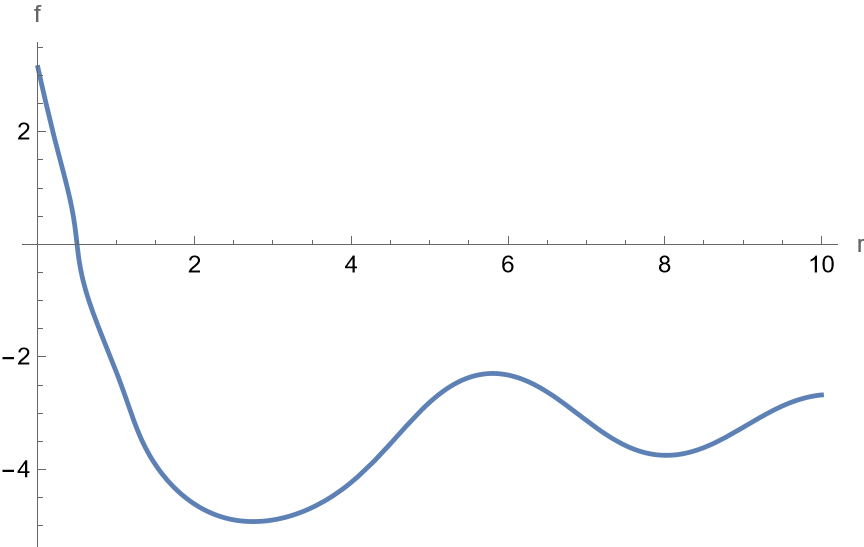
which doesn’t make any sense.

For the following discussions, I found paper arXiv:1309.1313 to be most helpful. Below are some approximation we can adopt at $r\to 0$,

\(\frac{\sin(f(r))}{r} \to f'(0), \quad \frac{1}{4}-\frac{\sin^2(f(r))}{r^2} -(f'(r))^2 \to \frac{1}{4}\) \(\frac{r^2}{4} + 2\sin^2(f(r)) = \frac{r^2}{4}\left( 1+8\frac{\sin^2(f(r))}{r^2} \right) \to \frac{r^2}{4}(1+8f'(0)).\)

Maybe we can make it work by providing a super accurate initial condition? With this hope I try to solve the equation at the origin, close to $r=0$. Expand $f(r)$ about the origin we get

where we have made use of the initial condition that $f(0)=\pi$, and $r$ is supposed to be very small. Take this to the equation of motion, with some manipulation we get

keep the leading order and NLO in $r$ we have

In paper arXiv:hep-ph/0106150v2, Ponchiano etc. adopted Pade approximation and it seems to be working good. But it’s not directly useful to me.

Well let’s move on to the next method.

The continuation (homotopy, embedding) method

The core idea behind the “continuation method” is that, instead of trying to solve a super-hard problem right away, we start with a simpler version of it that we can solve. Then, we “continue” from that solution, making small changes step by step, until we reach the solution of the original, harder problem.

1. Start Simple: Begin with a version of the problem that’s easy to solve.
2. Make Small Changes: Adjust the problem little by little, using the solution from the last step as the starting point for the next.
3. Reach the Target: Continue this process until you’ve transformed your simple problem’s solution into a solution for your original, harder problem.

Let us apply the aforementioned philosophical ideas into practice. Suppose we wish to solve a system of $N$ non-linear equations in $N$ variables, say

We assume $F$ is $C^{\infty}$. Suppose that we don’t know a lot about the initial value of the derivative, then we can’t effectively adopt the shooting method. As a possible remedy, define a homotopy or deformation $H(x,t)$ which deforms from some simpler equations $G(x)$ to $F(x)$ when $t$ smoothly changes, to be specific define

Everything is required to be smooth here. Typically, one can choose a so-called convex homotopy such as

$H(x,t)$ is the function we are trying to solve. Our job is to find $G(x)$ with known solution, then the PDE that $H(x,t)$ satisfies, offer the initial condition, then try to solve it.

Let’s look at an example. Let’s solve the following non-linear partial differential equation, which is a simplified version of the Ginzburg-Landau equation, a fundamental equation in superconductivity theory:

Here, $u(x, y, t)$ is the field we want to solve for, $\nabla^2 u$ is the Laplacian operator, $\lambda$ is a parameter, and $t$ represents time.

Let’s consider a square domain $[0, L] \times [0, L]$ with periodic boundary conditions. We will solve this equation using the continuation method by gradually increasing the parameter $\lambda$ and using the solution from the previous value of $\lambda$ as the initial condition for the next one.

This following code defines the PDE and its boundary conditions, then solves it using NDSolve for a range of values of $\lambda$, starting from $\lambda = 0$ and going up to $\lambda = 1$. The solution for each value of $\lambda$ is used as the initial condition for the next one. Finally, it plots the solution for $\lambda = 1$.

Here is the Mathematica code:

(* Define the domain size *)
L = 10;

(* Define the grid size *)
nx = 50;
ny = 50;

(* Define the time step and final time *)
dt = 0.01;
tmax = 1;

(* Define the initial condition *)
u0[x_, y_] := Sin[(Pi*x)/L] Sin[(Pi*y)/L];

(* Define the PDE *)
pde = D[u[x, y, t], t] == D[u[x, y, t], {x, 2}] + D[u[x, y, t], {y, 2}] + λ*u[x, y, t] - u[x, y, t]^3;

(* Solve the PDE using the continuation method *)
λvalues = Range[0, 1, 0.1];
usol = {};
uinit = u0[x, y];
For[i = 1, Length[λvalues], λ = λvalues[[i]];
  sol = NDSolve[{pde, u[x, y, 0] == uinit, 
    PeriodicBoundaryCondition[u[x, y, t], x == 0, TranslationTransform[{L, 0}]],
    PeriodicBoundaryCondition[u[x, y, t], y == 0, TranslationTransform[{0, L}]]},
   u, {x, 0, L}, {y, 0, L}, {t, 0, tmax}, 
   Method -> {"MethodOfLines", "SpatialDiscretization" -> {"TensorProductGrid", "MaxPoints" -> {nx, ny}}}];
  AppendTo[usol, sol];
  uinit = u[x, y, tmax] /. sol;
];

(* Plot the solution for λ = 1 *)
sol = usol[[-1]];
Plot3D[Evaluate[u[x, y, tmax] /. sol], {x, 0, L}, {y, 0, L}, AxesLabel -> {"x", "y", "u"}]

But before getting our hands dirty let’s consider another similar but different method, for reasons I’ll explain later.

The relaxation method

The term “relaxation” refers to the idea that an initial guess at the solution is iteratively refined or “relaxed” until it converges to the true solution.

Introduction to the Relaxation Method:

The relaxation method is often used for solving elliptic PDEs, such as Laplace’s equation and Poisson’s equation. The general approach of the relaxation method is as follows:

1. Discretize the domain of the PDE into a grid or mesh.
2. Make an initial guess for the solution at each grid point.
3. Iteratively update the solution at each grid point using a numerical approximation of the PDE.
4. Repeat step 3 until the solution converges to within a specified tolerance.

Let’s consider an example of solving Laplace’s equation on a rectangular domain $[0, a] \times [0, b]$ with Dirichlet boundary conditions.

Laplace’s equation is given by:

Where $u(x, y)$ is the function we are trying to solve for, and $\nabla^2$ is the Laplacian operator.

For simplicity, let’s consider the case where $a = b = 1$, and the boundary conditions are:

Here are the steps to solve this problem using the relaxation method in Mathematica:

(* Define the domain size *)
a = 1;
b = 1;

(* Define the grid size *)
nx = 10;
ny = 10;

(* Define the boundary conditions *)
u = Table[0, {nx + 1}, {ny + 1}];
Do[u[[1, j]] = 0, {j, ny + 1}];
Do[u[[nx + 1, j]] = 0, {j, ny + 1}];
Do[u[[i, 1]] = 0, {i, nx + 1}];
Do[u[[i, ny + 1]] = Sin[Pi*(i - 1)/nx], {i, nx + 1}];

(* Define the relaxation parameter *)
omega = 1.5;

(* Define the tolerance for convergence *)
tol = 10^(-6);

(* Perform the relaxation iteration *)
iteration = 0;
error = 1;
While[error > tol,
  error = 0;
  For[i = 2, i <= nx, i++,
    For[j = 2, j <= ny, j++,
      old = u[[i, j]];
      u[[i, j]] = (1 - omega)*u[[i, j]] + omega*0.25*(u[[i - 1, j]] + u[[i + 1, j]] + u[[i, j - 1]] + u[[i, j + 1]]);
      error = Max[error, Abs[u[[i, j]] - old]];
    ];
  ];
  iteration++;
];

(* Display the result *)
u

The u matrix contains the approximate solution to the PDE at each grid point. The While loop continues iterating until the maximum change in the solution at any grid point is less than the specified tolerance tol.

The relaxation method is a powerful and widely used numerical technique for solving PDEs. It is particularly well-suited for solving elliptic PDEs, such as Laplace’s equation and Poisson’s equation, which arise in various physical applications. The method is relatively simple to implement and can be easily adapted to different types of PDEs and boundary conditions.

However, it’s important to note that the convergence of the relaxation method can be sensitive to the choice of the relaxation parameter omega and the grid size. In some cases, it may be necessary to experiment with different values of these parameters to achieve a satisfactory solution.