Quartic time derivative in Lagrangian
Introduction
One day my postdoc supervisor handed me this function
\[T = \frac{\alpha}{2} b^{2}_ {i} + \frac{\beta}{4} (b^{2}_ {i})^{2}\]I guess $b_ {i}$ is something like $\dot{a}_ {i}$. $T$ is probably the kinetic energy.
The canonical momentum is
\[\pi_ {i} = \frac{\partial T}{\partial b_ {i}} = \alpha b_ {i} + \beta b^{2} b_ {i},\quad b^{2}:=b_ {i}b_ {i}.\]The question is, what is $T(\pi_ {i})$? And the next question, I guess, is how to quantize it?
There might be two methods adoptable here, Legendre transform and direct algebraic substitution. The latter is to solve for $b_ {i}$ from Eq.(5) and substitute it back to the expression for $T$.
The problem is that, the algebraic substitution will in general loose some information.
Functions are information. Different functions contain different functions, some contains more and some less. For example, the constant function contains little information. In general we have the following conclusions.
- The information of a function is equivalently contained in its graph. Thus, any operation that preserved the graph up to rotation, stretching, mirroring, etc. also preserved the information. For example, given a function $y=f(x)$, its inverse function, if exists, contains the same information since the graphs are just mirrored along $y=x$.
- The Fourier transform also preserves the information. In fact, functions are elements, or vectors in some Hilbert space and the Fourier transform corresponds to a change of representation.
So the question I wanna ask myself is, does Legendre transform preserve the information, just as Fourier transform?
Legendre transform
What is a Legendre transform, really? Given a function $y = f(x)$, or $y = y(x)$, sometimes we are more interested in the slope $dy / dx$, so much as to wanting them as the variable instead of $x$. So we define a new variable,
\[p:= \frac{dy}{dx} = p(x).\]Now how can we get a function in terms of $p$ without loosing any new information? The obvious way is to solve $x$ in terms of $p$, then substitute $x$ by $p$ in the original function to obtain $f(x(p))$. All seems good, except that this procedure actually causes a loss of information, as shown in the below example.
Consider a function $y =\frac{1}{2} (x-x_ {0})^{2}$, follow the procedure we introduced before, define
\[p := \frac{dy}{dx} = (x-x_ {0}) \implies x = p+x_ {0}\]take it back to the original function we get
\[y = \frac{1}{2} (p+x_ {0}-x_ {0})^{2} = \frac{1}{2}p^{2},\]$x_ {0}$ is gone! This is bad news since now we have loss the information of $x_ {0}$. Another way to say it is that, now two function with different $x_ {0}$ will be transformed to the same function $y=\frac{1}{2} p^{2}$. Bad news indeed. If it is a good transform, we should be able to transform it back to the original function, just as Fourier transform or Laplace transform or Borel transform, etc. Or, you could say now the information has been split to two places, the final function $\frac{p^{2}}{2}$ and the specific transform process, that is we used $p=x-x_ {0}$. Well, we don’t want the transform process itself to contain any information! When we are doing Fourier transform or anything, we don’t need to remember anything about the original function, do we?
Well there is a solution but only works for convex and concave functions. Recall that roughly speaking a convex function is a functions curves downwards and a concave function is a function that curves upwards. They are assumed to be almost-everywhere differentiable, if you don’t remember what “almost-everywhere” means please refer to my other notes.
Now, the solution of course is the Legendre transformation. Denote $\widetilde{y}$ the Legendre transformed function, we have
\[\widetilde{y}(p) = \begin{cases} \text{sup }\left\{ px - y(x) \right\} & y \text{ is convex}, \\ \text{inf }\left\{ px - y(x) \right\} & y \text{ is concave}. \end{cases}\]If the function is not convex/concave only in localized regions, then the transform still makes sense. Sometimes it is defined with an extra minus sign.
Let’s apply Legendre transform to $y=\frac{1}{2} (x-x_ {0})^{2}$, we have $p=dy / dx = x-x_ {0}$ and
\[\widetilde{y} = px-y = (x-x_ {0})x -\frac{1}{2} (x-x_ {0})^{2} = (x-x_ {0})\left( x-\frac{x}{2} + \frac{x_ {0}}{2} \right) = \frac{1}{2}(x-x_ {0})(x+x_ {0}),\]$x_ {0}$ is still there!
Now we can do the Legendre transform twice to prove that for certain functions
\[\widetilde{\widetilde{y}} = y.\]To show it, first perform once Legendre transform
\[\widetilde{y}(p)=p x(q)-y(q),\quad p = dy / dx.\]That is, assume you can solve for $x$ from $p$. Now, do it again we have
\[\widetilde{\widetilde{y}} = qp - \widetilde{y} = y(q)\]where I’ve omitted some details, but you can reproduce it, no problem.
Back to
\[T = \frac{\alpha}{2} b^{2} + \frac{\beta}{4} (b^{2})^{2},\quad b^{2}:= b_ {i}b_ {i}\]and the canonical momentum reads
\[\pi_ {i} = \frac{\partial T}{\partial b_ {i}} = \alpha b_ {i} + \beta b^{2} b_ {i},\quad b^{2}:=b_ {i}b_ {i}.\]Perform the Legendre transform to $T$ we get
\[H:= \pi_ {i}b_ {i}-T = \frac{\alpha}{2}b^{2} - \frac{3}{4}(b^{2})^{2}.\]So far it seems to lead to nowhere, so I’ll postpone the discussion on this matter. Now we directly jump to the algebraic substitution method. Does it cause any loss of information? If so, is the lost information important? I don’t know.
Algebraic substitution
So, let’s try to solve Eq. (5). Since only $\pi^{2}$ appears in the Lagrangian, we can square the equation on both sides
\[\pi^{2} = \alpha^{2}b^{2} + \beta^{2} (b^{2})^{3} + 2\alpha \beta (b^{2})^{2}\]This suffices as long as we don’t have to deal with $b_ {i}$ components individually. Let $t := \pi^{2}$ and $x:= b^{2}$ to simplify the notation we have
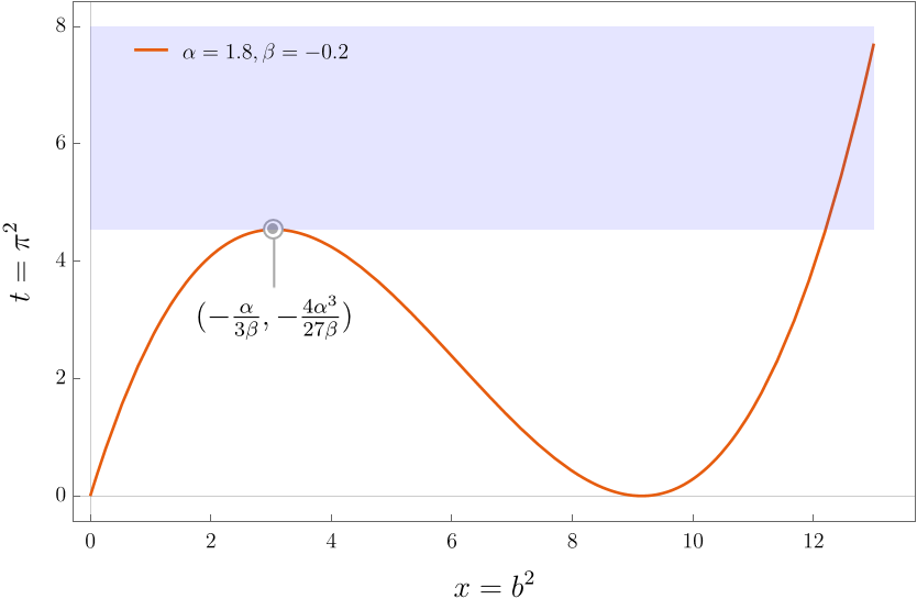
\[t = \beta^{2} x^{3}+2\alpha \beta x^{2}+\alpha^{2} x,\]which is
\[x^{3}+\frac{2\alpha }{\beta}x^{2}+\frac{\alpha^{2}}{\beta^{2}}x-\frac{t}{\beta^{2}}=0.\]Keep in mind that $x,t$ are positive by construction.
The graph of the right hand side of equation (6) can be illustrated using mathematica codes
Manipulate[Plot[\[Beta]^2 x^3 + 2 \[Alpha] \[Beta] x^2 + \[Alpha]^2 x, {x, 0, 15}, AxesLabel -> {"x", "t"}], {\[Alpha], -5, 5}, {\Beta], -5, 5}]
As the plot shows (also can be read-off from the equation itself), there is always the solution $t=x=0$. This is of no interests for us. What about the other root,which seems to be degenerate?
Equation (6) can be simplified to
\[t = \beta^{2} x \left( x+ \frac{\alpha}{\beta} \right)^{2}, \quad x,t>0.\]From this form things are much clearer, we see again $x=t=0$ is always a solution, there is another degenerate solution at
\[t=0,\quad x = - \frac{\alpha}{\beta}.\]Recall that we are only interested in $x,t\geq 0$, we will discuss to situations according to whether $\alpha$ and $\beta$ have the same sign or not.
1. $\alpha \beta\leq 0$
The local maximum is obtained at
\[x_ {\star } = - \frac{\alpha}{3\beta},\quad t_ {\star} = - \frac{4\alpha^{3}}{27\beta}.\]Thus there are three inequivalent real roots for
\[\alpha \beta < 0, \quad 0< t < -\frac{4\alpha^{3}}{27\beta},\]where if $t=0$ or $-4\alpha^{3} / 27 \beta$ then there will be two degenerate roots.
If
\[t > - \frac{4\alpha^{3}}{27\beta},\quad \text{one real root. }\]The situation is summarized in the plot below. The light blue area is where the real solution is unique to the cubic equation. We have marked the local maximum also.
2. $\alpha \beta> 0$
In this case, since $\alpha$ is fixed to be positive for physics reasons, $\beta$ is also fixed to be positive definite. From the graph it is easy to see that not there exist only one real root for $x=x(t)$ when both $x,t$ are required to be positive. The root formula gives by Mathematica reads
\[\begin{align} x =& -\frac{(-2)^{2/3}}{6 \beta ^2}\sqrt[3]{-2 \alpha ^3 \beta ^3+3 \sqrt{3} \sqrt{\beta ^7 t \left(4 \alpha ^3+27 \beta t\right)}-27 \beta ^4 t}\\ &\frac{\alpha}{3 \beta }\left(2-\frac{\sqrt[3]{-2} \alpha \beta }{\sqrt[3]{-2 \alpha ^3 \beta ^3+3 \sqrt{3} \sqrt{\beta ^7 t \left(4 \alpha ^3+27 \beta t\right)}-27 \beta ^4 t}}\right) \end{align}\]As a reminder to myself, you can’t always trust the factors of $i$ in the output of mathematica Solve command, sometimes the solution explicitly contains $i$ but it is actually real, sometimes the other way around. Numerical method is our best friend in this case.
The ancient way
The standard 16-th century approach. To really solve the cubic equation, we need to turn the equation to the the standard form, this equations reads
\[x^3+px=q\]where
\[\begin{align} p &=\frac{\alpha^{2}}{\beta^{2}} - \frac{1}{3}\left(\frac{2\alpha }{\beta}\right)^2, \\ q &=\frac{1}{3} \frac{2\alpha^{3}}{\beta^{3}} + \frac{t}{\beta} -\frac{2}{27}\left( \frac{2\alpha}{\beta} \right)^{3}. \end{align}\]According to some 16th century mathematics, we can then perform the so-called Vieta's substitution and get the three root. Vieta’s substitution reads
which reduces the equation to
\[w^{3}-\frac{p^{3}}{27w^{3}}-q =0\]which can be easily turned into a quadratic equation in $w^{3}$
\[(w^{3})^{2}-q(w^{3})-\frac{p^{3}}{27}=0.\]The quadratic formula says that
\[w^{3} = \frac{1}{2} q \pm \sqrt{ \frac{q^{2}}{4} + \frac{p^{3}}{27} }=: R\pm \sqrt{ R^{2}+Q^{3} }.\]Sometimes it is more useful to deal with $R$ and $Q$ instead of $p$ and $q$. There are therefore six (complex) solutions for $w$, which gives us three solutions for $x$.
Enjoy Reading This Article?
Here are some more articles you might like to read next: