Caratheodory's approach to Thermodynamics
Disclaimer: Nothing in this note is original. Including the figures.
Around 1909, Caratheodory was urged by Max Born to come up with an axiomatic treatment of thermodynamics. As a result, Caratheodory made use of Frobenius’s theorem and constructed a rather mathematical treatment of thermodynamics. In this note we will only superficially look at the theory.
Consider a system of fluids separated into $n$ chambers by “diathermous” membranes, namely membranes that allow only the passage of heat, not fluids, as shown in the figure below. Each chamber has its own pressure and volume, denoted by $p_{i}$ and $v_{i}$.
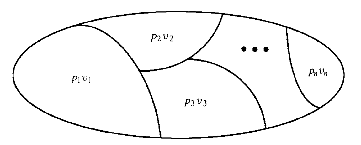
We assume that each state of the system is a thermal equilibrium state. We assume that the membranes are stretchy enough so that in the equilibrium state the pressure is uniform between different chambers, $p_{1}=p_{2}-\dots=p_{n}$. The equations of state (for instance, $p_{i}v_{i}=n_{i}RT$) will allow us to eliminate all but one pressure, say $p_{1}$. Then the state is described by $n+1$ parameters, $p_{1},v_{1},\dots,v_{n}$. The uniform temperature is given by the n-tuple from the equation of state. It is important to assume that there is a global internal energy function $U$ of the system that can be used instead $p_{1}$. The equilibrium state is then described by $n+1$ parameters,
Each $v_{0}$ will fix a point in the state space, namely the space of all the possible states. The state space then would be a $n+1$ dimensional manifold.
Next consider a sequence of states, forming a continuous change of the states, the change is slow enough that each state during the change is itself an equilibrium state. Such a slow change of states traces a curve in the state space. Such transition is sometimes called quasi-static.
We shall also consider non-quasi-static transitions, such as “stirring”. In the space of states, such a transition starts at some point $x$ and ends at some other points $y$, but since there is no sequence of equilibrium states intermediating the initial and final states, there is no path in the state space joining $x$ to $y$ (since each point in the state space represents a equilibrium state by construction). These corresponds to irreversible processes. Schematically, we shall draw such transitions by a dash line joining $x$ to $y$.
On the state manifold (the manifold of state space), we assume the existence of a work 1-form $W$, describing the work done by the system due to a change of volume.
Recall that when a form is closed, the integral of it along some boundary is always zero, thanks to the Stokes theorem. It is important to note that here the work 1-form $W$ is not supposed to be closed, thus if the system undergoes a loop of state transition, the total energy done by the system may not be zero. The line integral of $W$ is in general dependent upon the path joining the endpoint states.
We also assume the existence of a heat 1-form
representing the heat added or removed from the system. At first glance it seems strange that $Q$ should depend on $dv_{i}$, we will say more about it later. Again, $Q$ is not supposed to be closed, and we shall always assume that $Q$ never vanishes. Note that in some other texts $Q$ is derived, rather than postulated as here.
Remark. In some textbooks the 1-form $W$ and $Q$ are denoted by $d$ with a bar crossing the upper part, to show that they are different from usual $dQ$ and $dW$. It is very misleading, since that in the language of differential forms, $dW$ would be an exact form, but the work 1-form is in no means exact. The same goes for the heat 1-form.
The first law of thermodynamics says that
\[dU = Q-W.\]This is the conservation of energy.
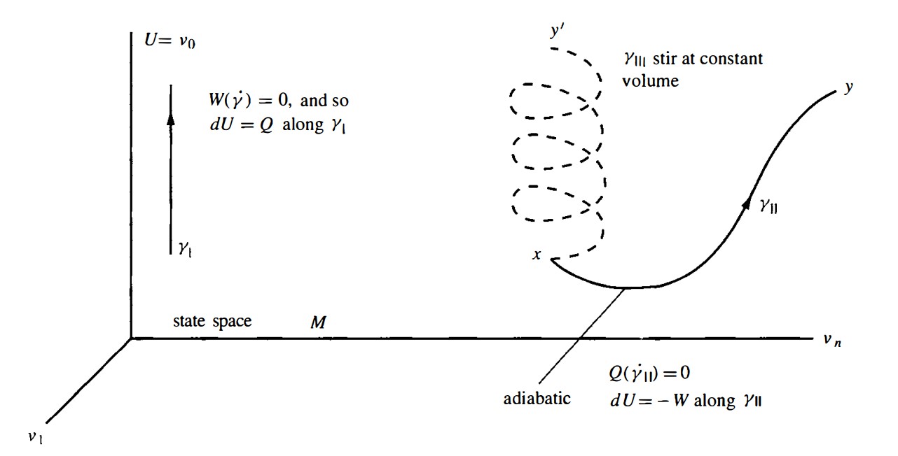
Next we show some elementary changes of states, and how the look like in the state space.
- Heating at constant volume. It is shown as $\gamma_{I}$ in the figure below. The work 1-form vanishes when evaluated on the tangent $\dot{\gamma}_{I}$. The conservation of energy says that $dU = Q$.
- Quasi-static adiabatic process. There is no heat added to the system, thus $Q=0$ along the path. It is shown by $\gamma_{I I}$.
- Stirring at constant volume. Since it is not quasi-static we cannot represent it by a curve in the state space. We can only schematically represent it by connecting $x$ and $y’$ with a dashed curve. $Q,W$ make no sense for this process.
Definition. A submersion is a smooth mapping $f:M\to N$ from an $m$-dimensional manifold $M$ to an $n$-dimensional manifold $N$, $m>n$, under which for any point $p\in M$, the map $f_{\ast}:T_{p}M\to T_{f(p)}N$ is onto.
A basic example of submersion is the so-called canonical submersion from $\mathbb{R}^{m}$ to $\mathbb{R}^{n}$ with $m>n$, given coordinate system $(x)$ on both the manifolds, the smooth mapping is defined by
\[f:(x^{1},\dots,x^{n},\dots,x^{m})\to (x^{1},\dots,x^{n}).\]The above figure suggests us to treat $U$ as a distinct dimension, separate it from the rest $v$ coordinates. We shall assume that there is a connected $n$-manifold (one dimension less than $M$, the state space), the mechanical manifold $V$. We assume there is a smooth map $\pi:M\to V$, which is a submersion. By the main theorem on submanifold, if $v\in V$ then $\pi^{-1}(v)$ is a 1-dimensional embedded submanifold of $M$. The manifold $V^{n}$ will be covered by a collection of local coordinates $v^{1},\dots,v^{n}$. $V$ takes the place of the volume coordinates used before. The curves $\pi^{-1}(v)$ corresponds to the heating and cooling at constant volume. Obviously on $\pi^{-1}(p)$ we have $W=0$. The $n+1$ tuple $U,v^{1},\dots,v^{n}$ forms a local coordinates system for $M$.
A cyclic process is one that starts and ends at the same state. The second law of thermodynamics, according to Lord Kelvin, can be stated as:
In no quasi-static cyclic process, can a quantity of heat be converted entirely into its mechanical equivalent of work.
The same law, according to Caratheodory(1909), says that
In every neighborhood of every state $x$ there are states $y$ that are not accessible from $x$ via quasi-static adiabatic paths, that is, paths along which $Q=0$.
It is not meant to be obvious, but Caratheodory’s assumption is weaker than Kelvin’s,
\[\boxed{ \text{Kelvin's assumption} \implies \text{Caratheodory's assumption.} }\]Take the path $\gamma_{I}$ in the previous figure for example, assume $\gamma_{I}$ goes form $x$ to $y$. If there were quasi-static and adiabatic process going from $x$ to $y$, call it path $\gamma_{I’}$, then along $\gamma_{I’}$ we would have
\[\int_{\gamma_{I'}} \, W = \int_{\gamma_{I'}} \,Q-dU = \int_{\gamma_{I'}} \,-dU=-\int_{\gamma_{I}} \,dU=-\int_{\gamma_{I}} \,Q\]where in the second-to-last step we changed from path to $\gamma_{I}$, which is allow since $dU$ is closed. But this would say that the heat energy pumped into the system has been entirely converted into mechanical work, which contradicts the Kelvin! Thus there is no such path $\gamma_{I’}$.
An adiabatic quasi-static process is a path in the state space such that $Q=0$ along it. We know that if $Q=0$ were a holonomic constraint, then there would exist other states $y$ in the neighborhood of $x$, that is not accessible from $x$ along any adiabatic path. All the accessible points would lie on the maximal leaf through $x$. The question is, does having inaccessible points in turn implies that the distribution $Q=0$ is integrable? Caratheodory showed that it is indeed the case. In the following we have a pure mathematical result:
Caratheodory’s theorem. Let $\theta$ be a 1-form which is smooth and non-vanishing on an $n$-dimensional manifold $M$, and suppose that $\theta=0$ is not integrable, thus at some point $x_{0}$ we have
\[\theta \wedge d\theta \neq 0.\]Then there is a neighborhood $U$ of $x_{0}$ such that any point $y$ in $U$ can be joined to $x_{0}$ by a piecewise smooth path that is always tangent to the distribution.
Roughly speaking, since $\theta=0$ is not holonomic, the distribution given by $\theta=0$ is not integrable, then at $x_{0}$, we can find two vectors $X,Y$ tangent to the distribution but their Lie bracket $[X,Y]$ is not in the distribution. They will allow us to move away from the distribution and reach any point $y$ in the neighborhood. A detailed proof can be found in Frankel.
We thus conclude from Caratheodory’s mathematical theorem, together with his version of the second law of thermodynamics, that the adiabatic distribution $Q=0$ is integrable.
If the reader is interested in the construction of entropy, one of the most important concepts in thermodynamics, from Caratheodory’s mathematical approach, please refer to Frankel and books referred therein.
Enjoy Reading This Article?
Here are some more articles you might like to read next: