Renormalization method in PDF
Abstract
The application of renormalization group method in solving the differential equation in the momentum space, and the error estimation of the solution with finite sized lattice size.
Introduction
The question we want to answer here is very simple: If we solve the PDF in the momentum space with a given cutoff $\Lambda$, how does the solution change with respect to $\Lambda$?
First Order Homogeneous Linear Differential Equation
We want a well behaved function $\mathbb{R} \to \mathbb{R}$ so we begin with Gaussian function $g(t) = e^{-\lambda t^2}$. The equation it solves is
\[\dot{g}(t) + 2 \lambda t g(t) = 0,\]which is a homogeneous first order ODE.
Imagine that the function is defined on a grid with lattice spacing $a$, then the equation takes the discrete form
\[\frac{g(t_ {i+1})-g(t_ i)}{a} + 2 \lambda t g(t_ i) = 0,\quad \forall i \in \text{ lattice},\]the solution will naturally depend on the lattice size, in the $a\to 0$ limit we will recover the continuous solution. We want to know what explicitly the dependence on $a$ looks like, and how to perform the error estimate with small but finite $a$.
As the first attempt, in our simplified example, we go to the frequency space by substitute
\[g(t) = \frac{1}{\sqrt{2\pi}}\int_ {-\infty}^{\infty} d\omega \tilde{g}(\omega) e^{-i\omega t}.\]The Fourier transformed equation reads
\[\int_ {-\infty}^{\infty} \frac{d\omega}{\sqrt{2\pi}} e^{-i\omega t} \left\lbrace -i \omega \tilde{g}(\omega) - 2i\lambda \frac{d}{d\omega} \tilde{g}(\omega) \right\rbrace.\]A lower bound in the lattice size $a$ corresponds to an upper bound $\Lambda$ in the momentum (exchangeable with frequency in our discussion) space, $a \sim 1/\Lambda$, thus we have
\[\begin{align} &\int_ {-\Lambda}^{\Lambda} \frac{d\omega}{\sqrt{2\pi}} e^{-i\omega t} \left\lbrace -i \omega \tilde{g}(\omega) - 2i\lambda \frac{d}{d\omega} \tilde{g}(\omega) \right\rbrace = 0, \\ \implies & \omega \tilde{g}(\omega) + 2\lambda \frac{d}{d\omega} \tilde{g}(\omega) = 0\, \forall \, |\omega| < \Lambda, \quad 0 \text{ otherwise} \end{align}\]The equation for $\tilde{g}(\omega)$ takes the same form (up to some multiplicative constants) as that for $g(t)$, reflecting the fact that the Fourier transformed Gaussian function takes the same form as the original function.
Here comes the key point: what happens if we decrease the momentum cutoff by infinitesimal, $\Lambda \to b\Lambda$, $b = 1-\epsilon$. With new cutoff $b\Lambda$ the equation above still holds trivially, since different modes are entirely independent of each other, we get
\[\omega \tilde{g}(\omega) + 2\lambda \frac{d}{d\omega} \tilde{g}(\omega) = 0\, \forall \, |\omega| < (1-\epsilon)\Lambda, \quad 0 \text{ otherwise}.\]In other words, for the modes that survive the renormalization flow, we have the trivial RG equation
\[\frac{d}{d\Lambda}\tilde{g}(\omega) = 0, \quad |\omega| < b\Lambda.\]Switch back to the physics space from frequency space, the error estimate is most easily done by subtracting $g^{(\Lambda)}(t)$ from $g^{(\infty)}(t)$, where
\[g^{(\Lambda)}(t) \equiv \frac{1}{\sqrt{2\pi}}\int_ {-\Lambda}^{\Lambda} d\omega \tilde{g}(\omega) e^{-i\omega t}\]where the Fourier transform of Gaussian function is
\[\mathcal{F}\left\lbrace e^{-\lambda x^2}\right\rbrace(\omega) = \frac{1}{\sqrt{2 \lambda }}e^{-\frac{\omega ^2}{4 \lambda }}\]Define
\[\boxed{\Delta g(t) \equiv g^{(\infty)}(t) - g^{(\Lambda)}(t)},\]we have
\[\begin{align} \notag \Delta g(t) &= \left( \int_ {-\infty}^{-\Lambda} + \int_ {\Lambda}^\infty \right) \left( \frac{d\omega}{\sqrt{2\pi}} \frac{1}{\sqrt{2\lambda}} e^{-\omega^2/4\lambda} e^{-i\omega t} \right) \\\notag &=\frac{1}{\sqrt{\pi\lambda}} \int_ {\Lambda}^\infty d\omega e^{-\omega^2/4\lambda} \cos{\omega t} \\\notag &= \frac{i}{2} e^{-\lambda t^2} \left(-2 i +\text{erfi}\left(\frac{-2 \lambda t+i \Lambda }{2 \sqrt{\lambda }}\right)+\text{erfi}\left(\frac{2 \lambda t+i \Lambda }{2 \sqrt{\lambda }}\right)\right)\\ &= e^{-\lambda t^2} - e^{-\lambda t^2}\text{Re}\,\text{erf}\left( \frac{\Lambda + 2i\lambda t}{2\sqrt{\lambda}} \right) \end{align}\]where we have simplified notations, Re erf is the real part of the error function, and $\text{erfi}(z)$ is the so-called imaginary error function defined by $\text{erfi}(z) = -i \,\text{erf}(iz)$.
Well, the last expression is not super helpful, we can do better by looking at $\Delta g^2$ as an estimate of the overall error. Square the second line in the previous equation we get
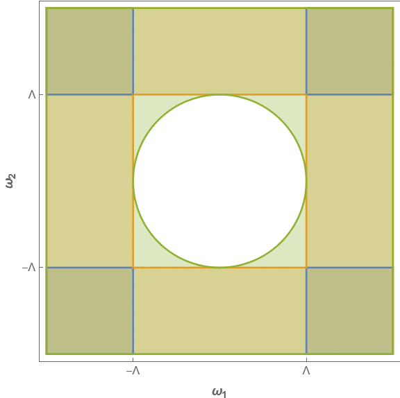
\[\begin{align*} \notag \Delta g(t)^2 &=\frac{1}{4\pi\lambda} \int_ {\left\lvert \omega_ 1 \right\rvert >\Lambda} d\omega_ 1 \int_ {\left\lvert \omega_ 2 \right\rvert >\Lambda} d\omega_ 2 \, e^{-\omega_ 1^2/4\lambda - \omega_ 1^2/4\lambda} \cos(\omega_ 1 t) \cos(\omega_ 2 t) \\\notag &=\frac{1}{4\pi\lambda} \int_ {\left\lvert \omega_ {1,2} \right\rvert >\Lambda} d^2\omega e^{-\omega^2/4\lambda} \cos(\omega_ 1 t) \cos(\omega_ 2 t) \\ & < \frac{1}{4\pi\lambda} \int_ {\left\lvert \omega_ {1,2} \right\rvert >\Lambda} d^2\omega e^{-\omega^2/4\lambda} \end{align*}\]where $\omega^2 = \omega_ 1^2 + \omega_ 2^2$. The integral region is shown in the Figure below, the four corners where $\omega_ {1,2}>\Lambda$ corresponds to the integral region. We can extend the region first to $(\mathbb{R}^2 - \text{square})$, then to $(\mathbb{R}^2 - \text{disk})$, each step will increase the error, thus we will get an upper bound. The reason for changing the square to circle is that so we can use the rotation symmetry. Continue with the integral,
\[\begin{align} \notag |\Delta g(t)|^2 &< \frac{1}{4\pi\lambda}\int_ {\omega^2>\Lambda^2} d^2\omega e^{-\omega^2/4\lambda}\\\notag &= \frac{1}{4\pi\lambda} \int_ {\omega^2>\Lambda^2} d^2\omega e^{-\omega^2/4\lambda} \\\notag &= \frac{1}{4\pi\lambda}2\pi \int_ {\Lambda}^\infty \int d\omega \, \omega e^{-\omega^2/4\lambda} \end{align}\]where we have used $d^2 \omega = d\omega \omega d\theta$,
\[\begin{align} |\Delta g(t)|^2 &< \frac{1}{4\lambda} \int_ {\Lambda}^\infty \int d\omega^2 \, \omega e^{-\omega^2/4\lambda} \\ &= e^{-\Lambda^2/4\lambda}. \end{align}\]The conclusion is that at each $t$, the error $[g^{(\infty)}-g^{(\infty)}]^2 < e^{-\Lambda^2/4\lambda}$.
Out of a more differential point of view, let us consider the change of the function as we vary the cutoff $\Lambda$. We can calculate $\boxed{\frac{d}{d\Lambda} g^{(\Lambda)}(t)}$. Note that sometimes we will neglect the independent variable $t$ to save some space.
If we increase $\Lambda$ infinitesimally, we have
\[\begin{align} \notag g^{(\Lambda+\epsilon)}(t) & = g^{(\Lambda)} + \frac{1}{\sqrt{\pi\lambda}} \int_ \Lambda^{\Lambda+\epsilon} d\omega e^{-\omega^2/4\lambda} \cos(\omega t)\\ &= g^{(\Lambda)} + \frac{\epsilon}{\sqrt{\pi\lambda}} e^{-\Lambda^2/4\lambda} \cos(\Lambda t), \end{align}\]Thus
\[\boxed{ \frac{d}{d\Lambda} g^{(\Lambda)}(t) = \frac{e^{-\Lambda^2 / 4\lambda}}{\sqrt{\pi\lambda}} \cos(\Lambda t) = \text{Re}\,\frac{e^{-\Lambda^2 / 4\lambda}}{\sqrt{\pi\lambda}} e^{i\Lambda t} = \text{Re}\,\frac{e^{-\lambda t^2}}{\sqrt{\pi\lambda}} e^{-\frac{1}{4\lambda} (\Lambda-i2\lambda t)^2}. }\]It can be solved to give,
\[g^{(\Lambda)}(t) = C_ 1 - e^{-\lambda t^2} \text{Re} \, \text{erf}\left(i\sqrt{\lambda} t - \frac{\Lambda}{2\sqrt{\lambda}}\right),\]where $C_ 1$ is the constant of integration. To eliminate $C_ 1$, recall that $f^{\infty}(t) = e^{-\lambda t^2}$, thus we have $C_ 1 = 0$. By the end of the day we have
\[\boxed{ g^{(\Lambda)}(t) = - e^{-\lambda t^2} \text{Re} \, \text{erf}\left(i\sqrt{\lambda} t - \frac{\Lambda}{2\sqrt{\lambda}}\right) },\]which agrees with the previous equations. The value of $\Delta g(t)$ can also be estimated with the help of Hans Heinrich Burmann’s theorem,
\[\text{erf}{x} = \frac{2}{\sqrt{\pi}}\text{sgn}\cdot \sqrt{1-e^{-x^2}} \left( \frac{\sqrt{\pi}}{2}+ \sum_ {k\in \mathbb{Z}^+} c_ k e^{-k x^2} \right), \, c_ 1 = \frac{31}{200},\, c_ 2 = -\frac{341}{8000},\, \cdots.\]In summary, We have obtained the lattice spacing dependence, or equivalently the momentum cutoff dependence, both the error estimate and the RG flow are discussed.
In-homogeneous Linear Differential Equation
kink Equation
Conventions
The conventions are chose so be the same as that used by Mathematica.
Given a function $f(t):\mathbb{R} \to \mathbb{R}$, the Fourier transform in the symmetrical form is
\[\begin{align} \tilde{f} (\omega) &= \frac{1}{\sqrt{2\pi}}\int_ {-\infty}^\infty f(t) e^{i\omega t} dt, \\ f(t) &= \frac{1}{\sqrt{2\pi}}\int_ {-\infty}^\infty \tilde{f}(\omega) e^{-i\omega t} dt \end{align}\]where $\tilde{f}(\omega) \equiv \mathcal{F} \left\lbrace f \right\rbrace(\omega)$.
Note the factor of $\frac{1}{\sqrt{2\pi}}$ and the signs in the exponent.
Appendix A. Error function in the complex plane
The error function in the complex plane is defined to be
\[\operatorname* {erf}{z} = \frac{2}{\sqrt{\pi}} \int_ {\Gamma} d\zeta \, e^{-\zeta^2}\]where $\Gamma$ is any path going from $0$ to $z$. The real and imaginary part of an error function can be estimated by Abramowitz and Stegun.
The error function $\text{erf}(z),\, z \in \mathbb{C}$ satisfy symmetry relations
\[\begin{align} \text{erf}(z) &= - \text{erf}(-z), \\ \text{erf}(\overline{z}) &= \overline{\text{erf}(z)}. \end{align}\]A possibly useful series expression for numerical calculation is
\[\begin{multline} \operatorname* {erf}(x+i y) = \operatorname* {erf}{x} + \frac{e^{-x^2}}{2 \pi x} [(1-\cos{2 x y})+i \sin{2 x y}]\\ + \frac{2}{\pi} e^{-x^2} \sum_ {k=1}^{\infty} \frac{e^{-k^2/4}}{k^2+4 x^2}[f_ k(x,y)+i g_ k(x,y)] + \epsilon(x,y) \end{multline}\]where
\[\begin{align*} f_ k(x,y) &= 2 x [1-\cos(2 x y) \cosh(k y)] + k\sin(2 x y) \sinh(k y), \\ g_ k(x,y) &= 2 x \sin(2 x y) \cosh(k y) + k\cos(2 x y) \sinh(k y). \end{align*}\]Enjoy Reading This Article?
Here are some more articles you might like to read next: